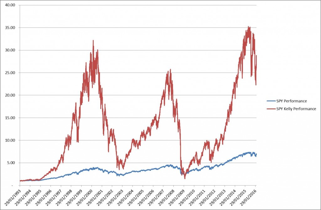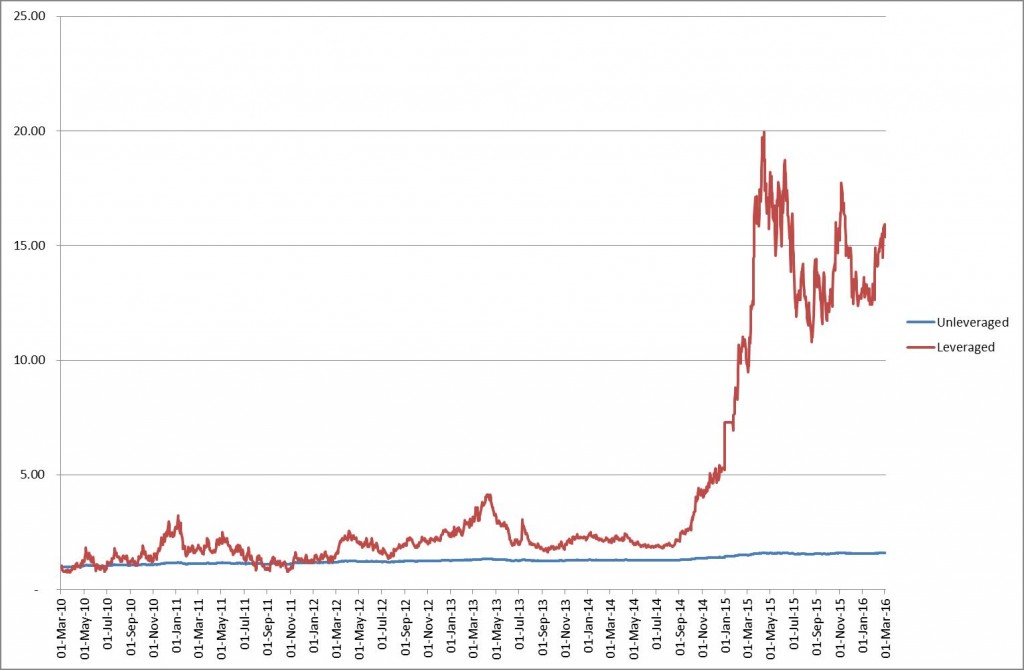
Kelly betting is an optimal approach to allocating capital to your system. In this article I want to show you how to apply this approach to your trading, and more importantly what kind of interesting questions you can answer using the ideas behind Kelly betting, in particular: “How long does it take to double my money?”
First let’s start out with a simple example and progress to actual markets and trading systems.
The example is as follows, and tends to be an interview question for applicants to the financial industry. If I have a coin which lands heads with 60% probability and tails with 40%, how much should I bet on each go to make the most amount of money, assuming I start with $1000? Where for arguments sake you have N goes, and you can let N be as big as you want.
As always the devil is in the detail, and you need to be precise with your definitions. If you go down the route of interpreting the question as to maximizing terminal wealth, that is having the most amount of money available after you have N goes, you end up with the mathematically sound, but intuitively wrong answer: bet everything on each go.
Why? Well, because there is a good chance (given the odds are stacked massively in your favour) that you will be right on every go of your coin-flip. Therefore the only way of making the most money possible, is to bet everything. Of course, there is the chance that you are wrong on one go, and that’s the end of the game. You lose. That’s the counterintuitive bit.
So maybe the question is wrong. Rather than asking “how to get to the most amount of money at the end of the game,” you should ask how to ensure that my money grows the fastest. This form of question takes the probability of losing everything on one go, if you bet everything, into account.
In essence you are optimizing the growth-rate of your money, and not your terminal wealth. In this simple game you can, after some algebra, work out the fraction of money you need to bet on every single toss of a coin, and the fraction of your money is the Kelly criterion, and depends on the probabilities of the outcomes of Heads or Tails.
Now we can ask if there is a similar approach to trading systems and markets. The answer is yes, and takes a similar approach, though it is important to understand the underlying assumptions that are being made.
Let’s start, and give some examples as we go along.
Let’s look at the S&P500 first. The easiest way of participating is to buy the SPY. It’s and ETG that tracks the index and whose price is a tenth of the index value. Let’s say that you use a leverage of 1x, so that you fully fund your SPY holding. The question we need to ask: is this the right amount of leverage to use? Let’s say that we could use leverage (via CFDs for instance), how much should the leverage be?
Before we proceed to answer that question, note that one key assumption we are making here is that the return statistics of the SPY are stable and constant, similar to the coin probabilities before. Otherwise, our leverage ratio would be changing on a daily basis. One way to achieve this is to estimate our ratio over sufficient long periods of time (we’ll get to which stats in a second).
The next implicit assumption is really important, and one of the key components of Kelly. This constant leverage ratio DOES NOT imply a constant position size!! If you are leveraged 2x, let’s say, then assuming you had a loss day, yesterday, your position size needs to decrease on the next day. If you were to keep the position size the same, then the P&L volatility would be bigger than a 2x leverage.
Let’s use some numbers to make this clear. Let’s say you are 2x leveraged and you have $1,000 capital. So you buy $2,000 worth of S&P. Let’s say the S&P goes down by 2%, so you incur a loss of $40. Your new capital is now $960. At 2x leverage this would give you an exposure of $1920 worth of S&P on the next day. However your original position size is worth $1960. So you have to reduce your position size. Kelly does mean daily rebalancing.
Ok, so how do you go about figuring out the optimal leverage? The simplest way is to use a spreadsheet. Here is a link to one that includes the SPY calculation:
[wpdm_package id=’628′]
You can look at the formulas and see how changing the leverage factor ultimately changes the overall growth rate.

So how does this apply to your trading?
Your trading strategy is nothing more than an asset that generates daily returns. So you can write down your daily P&L in a spreadsheet. Be careful that you don’t mix apples and oranges. For starters if you are trading various systems, separate them out. You could equally separate out the P&L for each individual currency. Further you should record only your pip P&L, rather than your dollar P&L. Why? This removes the varying position sizes you might have applied. You want to find out the optimal size given your system, and if you muddy the waters with some previous sizing you’ve used you won’t get the right answer.
Once you’re done write down the daily P&L that you’ve experienced for each system/currency pair you’ve traded. This is an important step. It introduces the notion of time. The Kelly criterion itself has no notion of time, but it makes no sense to estimate statistics based on trade count. Why? Since as humans we want to have a handle on the speed of our wealth growth, and trade count doesn’t make that transparent.
Once you’ve done all that you can use following formula to figure out your right leverage:

You can find the implementation in the spreadsheet above:
[wpdm_package id=’628′]
where the numbers come from a straight-forward London Open Breakout strategy. Note that this Kelly criterion is actually the Sharpe Ratio divided by the standard deviation of returns. And indeed it is independent of the units of time we use.
In plain language μ, the top part of the Kelly criterion fraction, K, is the average daily return, and σ, the bottom part, is the standard deviation of daily returns.
For the London Breakout strategy we find this Kelly criterion to be 10x leverage.

Now to some caveats in using the Kelly criterion. As you can see we derived it by using historical data. So what happens if the historical criteria change? Well the one thing that can happen is that given new data, the estimated Kelly criterion decreases. The one thing we need to remember is that the Kelly criterion gives you the maximum leverage you can use without going bankrupt, i.e. overleveraging. So if the market changes, it could well be that your old Kelly criterion is now completely overestimated, compared to the real market dynamics, and you are running real risk of blowing up. Aside from that, Kelly is very aggressive. It does imply that you can experience drawdowns which are sizeable, in excess of 50%, sometimes even more.
For these reasons, people tend to argue in favour of using a fraction of the Kelly criterion.
Also note that Kelly is not the same as betting a certain amount of your capital, like 1% per trade (assuming you have a stop on your trades). All Kelly says, is that assuming your returns are generally well-behaved, and you have an edge, you need to keep a certain amount of leverage on your portfolio, and increase your position as you make money, and decrease it as you lose.
Now to the interesting question at the start of this article. How long does it take to double your money? In our case, how long assuming you use Kelly? This question was also the reason we introduced our daily measurement, so that we can have a unit of time attached to our answers.
To answer this question, we can work it out from the complex formulas used for deriving Kelly for market conditions; or we can use simulations. Regardless, here are the answers for a number of parameters:
| Kelly Fraction | Sharpe Ratio | Time in Years |
|---|---|---|
| Full Kelly | 0.5 | 2.8 |
| Half Kelly | 0.5 | 5.5 |
| Full Kelly | 1.0 | 0.75 |
| Half Kelly | 1.0 | 1.4 |
| Full Kelly | 1.5 | 0.35 |
| Half Kelly | 1.5 | 0.6 |
| Full Kelly | 2.0 | 0.2 |
| Half Kelly | 2.0 | 0.35 |
We should put several things into perspective here. The S&P500 has a long run Sharpe of 0.5. And indeed a full Kelly would have yielded 3000% in the last 6 years. Much more than the 100% we are looking for. So you need to take the averages here with a wide margin of confidence. Secondly achieving a Sharpe Ratio of 1 is feasible. Just read a book on the Turtles and do it yourself. Or look at Dual Momentum, or follow my currency FX Benchmark. A Sharpe Ratio of 1 is also considered A-Grade investment material in the majority of the investment community. A Sharpe Ratio of 2 or higher is indeed “God”-like investment abilities, which is evidenced by the quickness of doubling your money. But here is the crux of the matter: if you can double so quickly, shouldn’t you be the richest man in the world? NO! Of course not. By using high leverage your position size becomes very big. And any high Sharpe ratio will be eroded immediately. These things tend to be so high because of small position sizing and efficient execution.
This goes back to the old adage, it’s easier to double or even ten-fold your money when you don’t have that much. When you have $1bn dollars, try buying that much worth of lumber, or that much worth of IBM shares without moving the market against you!
You can use the attached spreadsheet and your own P&L record to work out your Sharpe Ratio, and from that deduce the various outputs. To get a decent confidence around these estimates you will need a good number of observations. At least six months of trading should help you figure out the answer to the question “How Long to Double My Money.”
If you have enjoyed this post follow me on Twitter and sign-up to my Newsletter for weekly updates on trading strategies and other market insights!

Hi Corvin,
great material! I have a question : I was looking at the Kelly spreadsheet, the London Breakout strategy. It seems, if I understand correctly that unleveraged is always betting 0.1 lots and levereraged 10 times more 1.1
but in real life people always bet a percentage of the account, either equity (unleveraged) or free margin (leveraged)… , if the account has 10.000 in equity and it goes does down to 9.000 even unleveraged lot size should be reduced …I don’t understand in the example seems to be always fixed?
Hi Peter,
Thank you for your comment! There is a slight logical inconsistency in the spreadsheet, which ties in with your remark. Let me explain.
The approach I intended to take was to have a fixed notional and look at the daily returns on this fixed notional, in this case 10,000. This would actually mean working out the strategy returns on fixed lot size of 0.1 with respect to a fixed 10,000 notional, rather than the running notional. I have fixed this and uploaded the new version of the spreadsheet.
Now, with regards to your comment on having the original strategy de-leverage automatically on drawdowns: this adds a layer of money-management on top, which is feasible, but makes the issue more complicated. An underlying assumption of Kelly (in its standard form), is that the returns of the strategy are not dependent day-on-day from each other (i.e. serially un-correlated). And from this point of view (regardless if the assumption is correct or not), you derive the Kelly criterion.
Of course you could work into your initial strategy this deleveraging assumption, and then re-work your returns and derive a new leverage factor from there. This just goes over to the next order of complexity. Ultimately Kelly seeks to optimize for the maximum compound growth, and once you have your original return series, it allows you to play around with the leverage criterion until you obtain an equity curve that corresponds to your risk appetite.
Thank you for raising this question!
Hi Corvin!
many thanks for your detailed reply and updating the spreedsheet!
I saw the updated spreadsheet, now the returns are calculated by dividing the pips by 10.000 always, so 68 pips will always be the same return no matter the value of the account at the time, I understand that.
when I say that position sizing adjusts to the account value, maybe I didn’t made my point clear, I can try again:
kelly is 9.06 so for every 10.000 in the account unleveraged the lot size is 0.1 and leveraged should be 0.9 lots…
lets say the account grows to 20.000, my understanding is that now the unleveraged should be 0.2 lots and leveraged should be 1.8
and if the account goes to 5.000 unleveraged lot size should go to 0.05 and leveraged 0.45
nothing do to with the distribution of the returns, but only to to with the size of the notional account
Krgds