
At last! We’ve made it to the mean-reverting part of the series, starting with our focus on equities and their mean-reversion habits.
So, here’s the deal. We’re going to keep it simple, just like in the previous three posts, and start from the ground up. Over the following series we’ll culminate in a simple, straightforward (and well known) system that still works.
In detail for this article:
- What do we mean by mean-reversion and how can we measure it?
- What are some natural methods to trade this?
- We’ll look at the results from these naïve setups!
Be fore-warned, there won’t be any rinky-dink magic marker indicator at play here. It’s actually really easy to set up. So if you think only magic grails will do it for you, you gotta move one.
Also, mean-reversion doesn’t exist only in equities, but in other asset classes as well. We’ll get to those topic in the follow-up articles. Those will also include the Python code (and spreadsheets) to go along with these examples.
What’s Mean-Reversion, and How Can We Measure It?
Let’s start out with some basic stats.
You see, any time-series (that is a price-series in our trading parlance), has several basic properties (which are relevant to our discussion):
- Drift (aka mean)
- Swing-around (aka standard deviation)
- Bias towards negative or positive outcomes (skew)
- Dependency upon previous returns (auto-correlation)
The first are known as the first three moments (usually expressed as \(\mathbb{E}X^{1,2,3}\)), and tell you about the likelihood of a day’s return.
The last one, the autocorrelation gives you some forecasting power, as it tells you on average what happens tomorrow given today’s price behaviour. The sign here is important. If the auto-correlation is negative it means that if we had an up-day, it’s more likely we’ll have a down-day next.
To figure out if we have some sort of mean-reversion going on, we’re also going introduce time in our equation.
In particular different time frequencies. Remember Alexander Elder’s Triple Screen Trading System? It advocated looking at various time-frames to identify the asset’s behaviour.
Well, we’re going to do exactly focusing on daily, weekly, and monthly equity returns.
And to keep the article to the point: by equity I mean the S&P 500 market.
So here are the stats for the Daily, Weekly, and Monthly returns of the S&P 500:
| Daily | Weekly | Monthly | |
|---|---|---|---|
| Mean | 10.0% | 10.0% | 10.0% |
| StDev | 17.8% | 16.4% | 14.2% |
| Skew | 0.10 | -0.6 | -0.7 |
| Auto Corre | -6.3% | -8.5% | 6.3% |
Here is how we interpret the numbers:
We see that for monthly returns the auto-correlation is positive. And this is exactly what we exploited in the previous articles.
For Weekly and Daily returns we have negative auto-correlation which indicates that returns tend to want to go the opposite way.
So over the short time-horizon we can expect some form of whip-sawing.
What is definitely important to note is that the whip-sawing as measured over the various timescales isn’t the same. The standard-deviation actually becomes smaller over longer time horizons. This is an example of a Variance-Ratio test applied to a price-sers.
This result indicates that we expect our price-series to mean-revert, as the shorter time horizon swings need to be constrained strongly to give a lower volatility over longer time-horizons.
Furthermore, on the dailies, we see that the skew is positive. What this means for the case we are investigating is interesting: only on the daily returns do our daily returns actually overshoot the down days. If we look at the max / min of the daily, weekly, monthly returns we get:
| Daily | Weekly | Monthly | |
|---|---|---|---|
| Min Return | -10% | -20% | -17% |
| Max Return | 15% | 13% | 11% |
So the stats imply that over short time horizons we expect returns to go against the previous direction, which ultimately is the essence of mean-reversion. And we should focus on the dailies, where a positive skew, a positive drift will add a double whammy after we experience dips.
This is in accordance with an important observartion for our sample period: the equity markets were strongly upward trending (1993 to 2017). And as we saw previously this is a phenomenon that goes back even further. It’s important to note, because we can ex-ante expect long positions to outperform short positions!
Two Ways to Trade Equity Mean Reversion
Given the picture we’ve painted above here are two ways that immediately come to mind if you want to trade mean-reversion:
- If the market has been going in one direction, go the other way
- Trade in the opposite direction to the market’s short term directional trend.
We’re going to implement these approaches on daily closes. And for these two cases, we’ll focus on only trading until the close of the next day.
Nothing revolutionary. However, you immediately outperform the equity market by a wide margin! Actually on a par with some of the biggest money managers and hedge funds out there.
In detail:
Case 1: If the market has been going down for N straight days, buy at the close and hold for one day.
It’s pretty naïve, but we are not too concerned right now with being sophisticated.
In-line with our expectations above, going short really only helped throughout the 2008 collapse. So, we’ll scrap that side of the equation.
We’ll also focus on N = 1 for the time being. Let’s not give anybody the chance to claim I’ve been data snooping! (I have, but the results are stable).
Case 2: If the market is below its 5-day moving average, buy on the close and hold for one day.
Again, we’ll drop the short side of the equation.
The reason we chose 5-days is because it fits the fact that we see mean-reversion already kick in over the spane of a week: look at the compression of volatility over that period.
Drum Roll: The Results
Case 1: Buying after a down day
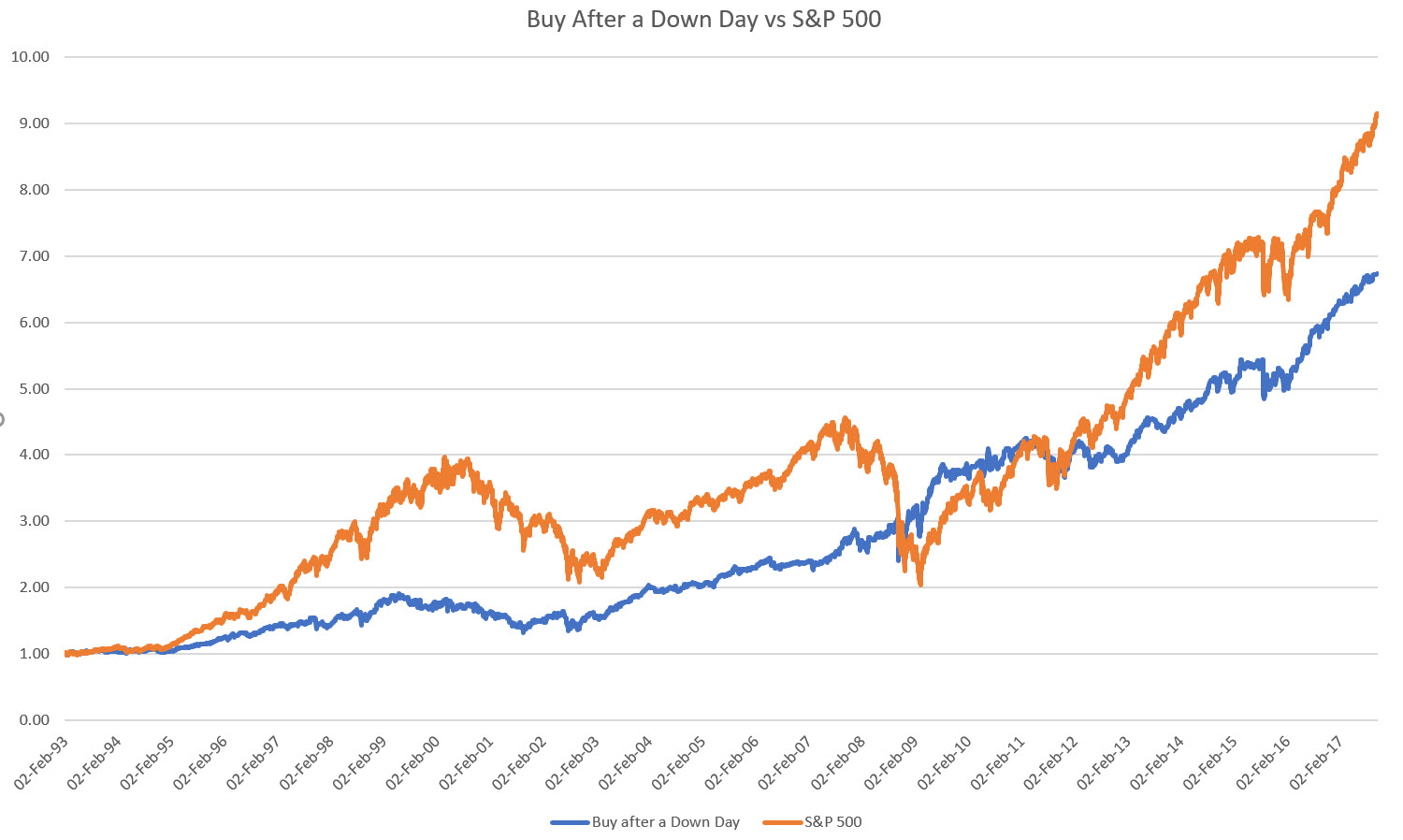
You might say, “no-way,” you’re making less!
But hang-on. Don’t you see that your draw-downs are lower, and the equity curve is smoother? Let’s measure that:
| Down Day | S&P 500 | |
|---|---|---|
| Ann. Returns | 8.7% | 10.7% |
| Ann. Volatility | 13.8% | 18.4% |
| Sharpe Ratio | 0.63 | 0.58 |
| Max D/D | -31% | -55% |
And now let’s take on a similar risk to the S&P 500 on our trading strategy.
Specifically we’ll just match the drawdown!
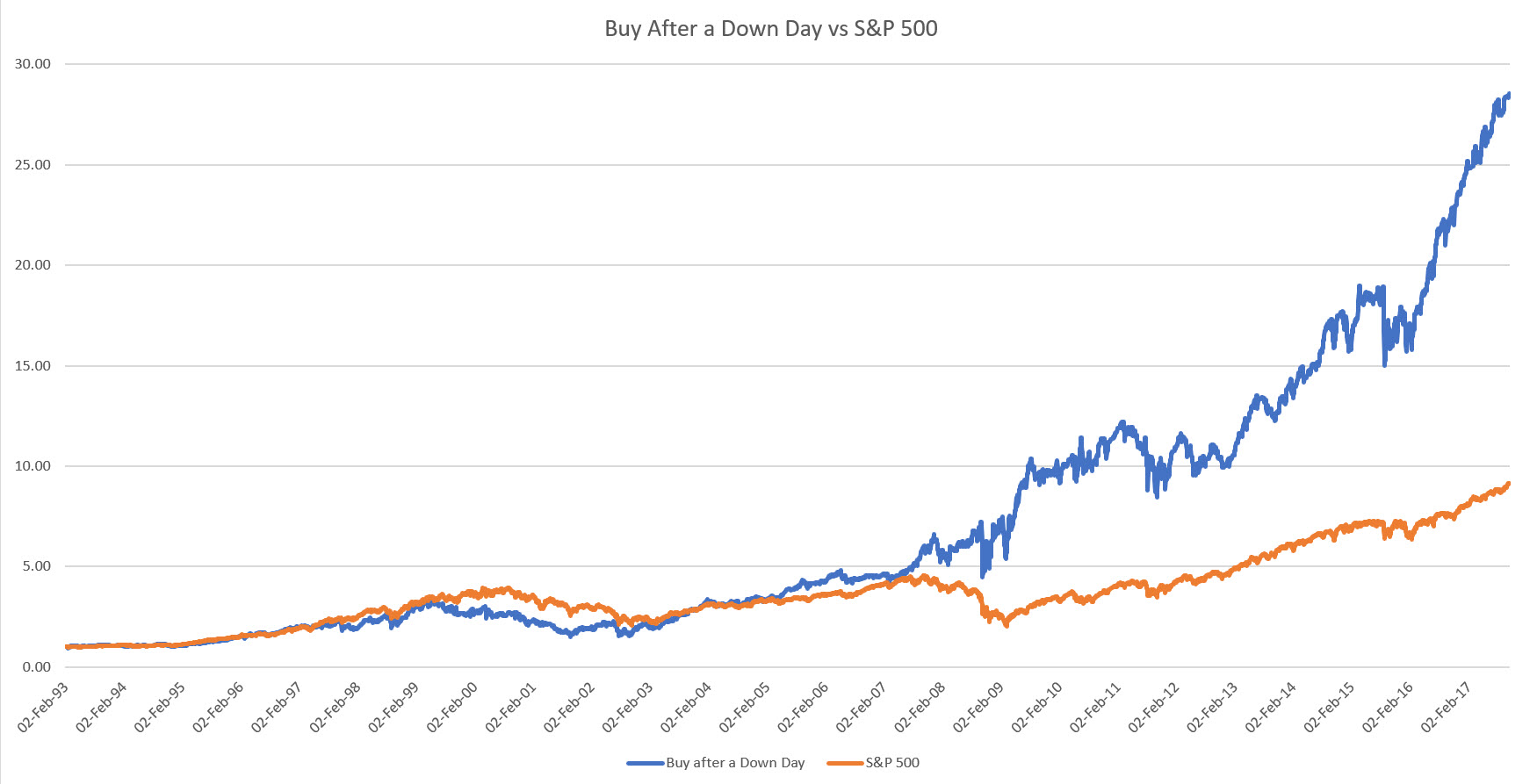
This is a CAGR of 27%. Certainly a good return. You might squabble over the Sharpe Ratio not being close enough to 1 but we’ll deal with that later.
Case 2: below the 5-day moving average
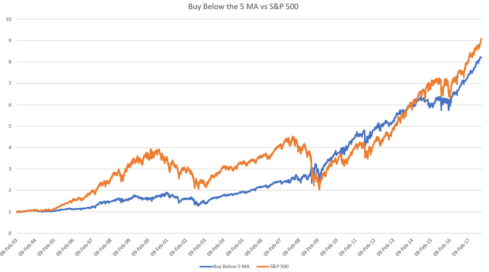
We get a similar performance as for Case 1. Again we can list out the stats:
| Down Day | S&P 500 | |
|---|---|---|
| Ann. Returns | 9.6% | 10.7% |
| Ann. Volatility | 14.3% | 18.4% |
| Sharpe Ratio | 0.67 | 0.58 |
| Max D/D | -33% | -55% |
And again we can scale up to get the same risk as the S&P 500 as measured in terms of its drawdown:
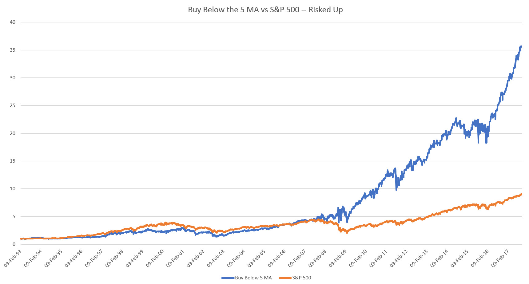
For Case 2 we also hit it out of the ball park with a 27% return on an annualized basis!
Systems Combined
We can now rightly ask what happens if we combine the two concepts? That is, buy after a down day, and close out once we hit the 5 day moving average (or cross above it).
The rationale? Mean-reversion complete.
We buy after we drop, and we close out after we hit the weekly mean. I.e. we revert to the mean in the true and proper sense of the word.
It turns out that by keeping the memory length to only one day as a decider for our buying strategy is too short, and gets swamped by the moving average overlay. We therefore need to extend it to the next logical step: buy when we have experienced a two day drop.
On an unleveraged basis we managed to improve performance. Here are the stats for this approach:
| Full Mean-Reversion | S&P 500 | |
|---|---|---|
| Ann. Returns | 9.1% | 10.7% |
| Ann. Volatility | 13.0% | 18.4% |
| Sharpe Ratio | 0.7 | 0.58 |
| Max D/D | 24% | -55% |
We have pushed the Sharpe up to 0.7. But what’s remarkable now is that our drawdown has decreased to 24%. So let’s risk this up so that we match the S&P 500 in terms of drawdowns:
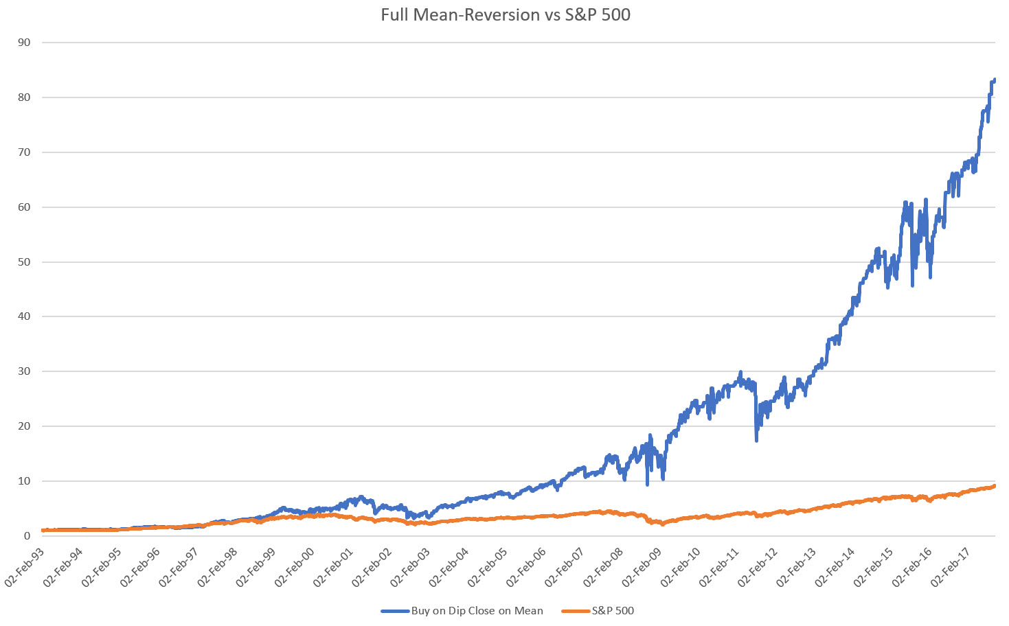
We now get a 34% CAGR. Trust me, this is indeed something to write home about!
Recap
In this article we covered set some of the foundational details of developing trading systems. In particular we looked at mean-reversion:
- How to measure and define it
- Two naïve approaches to trading it
- Combining the two ideas to hit the definition of reverting to the mean
- Seeing that the end result puts you in the top league of hedge fund managers
Do you still believe that trading is difficult?
Imagine combining this strategy with our momentum strategy, what would happen then…?
See You Next Time…
Next time we’ll take a stab at improving our mean-reversion approach by looking at some of the favourite indicators out there in combination with our rule-set above.
The end result is pretty impressive, as it extends the Sharpe Ratio we’re encountering from 0.7 to 1.0, and the resulting performance is truly astounding.
Surprisingly this particular system has been well-known for some time, and I’ve traded it for several years consistently. I’m highlighting this in case people start to moan about curve fitting and data snooping.
So, try to replicate these calculations, and see if you can repeat the performance.
Until next time,
Happy Trading.
If you have enjoyed this post follow me on Twitter and sign-up to my Newsletter for weekly updates on trading strategies and other market insights below!

Leave a Reply