Dangers of Backtesting, Over-Leverage and the Need for a Protective Stop

Backtesting and Over-Leverage are the bane of any systematic trader.

A shout out to Peter who raised both these points on the previous article in the series: Trading Numbers

So, what are the two issues we’ll address in this week’s article:

• Look ahead bias, and is it really that bad?
• Kelly is always touted as optimal. Is it really that optimal?

And to all those who don’t like spoilers: (2) will be covered in more detail later in this article series, so close your eyes; but following Peter’s comments, I couldn’t help include some detailed analysis here, I hadn’t really considered earlier.

Backtesting and Look Ahead Bias

I hear you asking, “What’s this look under the bed bias??”

Well, remember in Trading Numbers, we used momentum to setup a strategy that easily outperformed the S&P500.

Recapping: on the last trading day of the month you looked back over the last year.  If the S&P500 had finished up, you bought, otherwise you were flat.  Nice and simple.

Now assume that you were a bit sloppy implementing this in your spreadsheet, and you let a Look Ahead bias creep in.  Let’s see what this bias could have led us to believe:

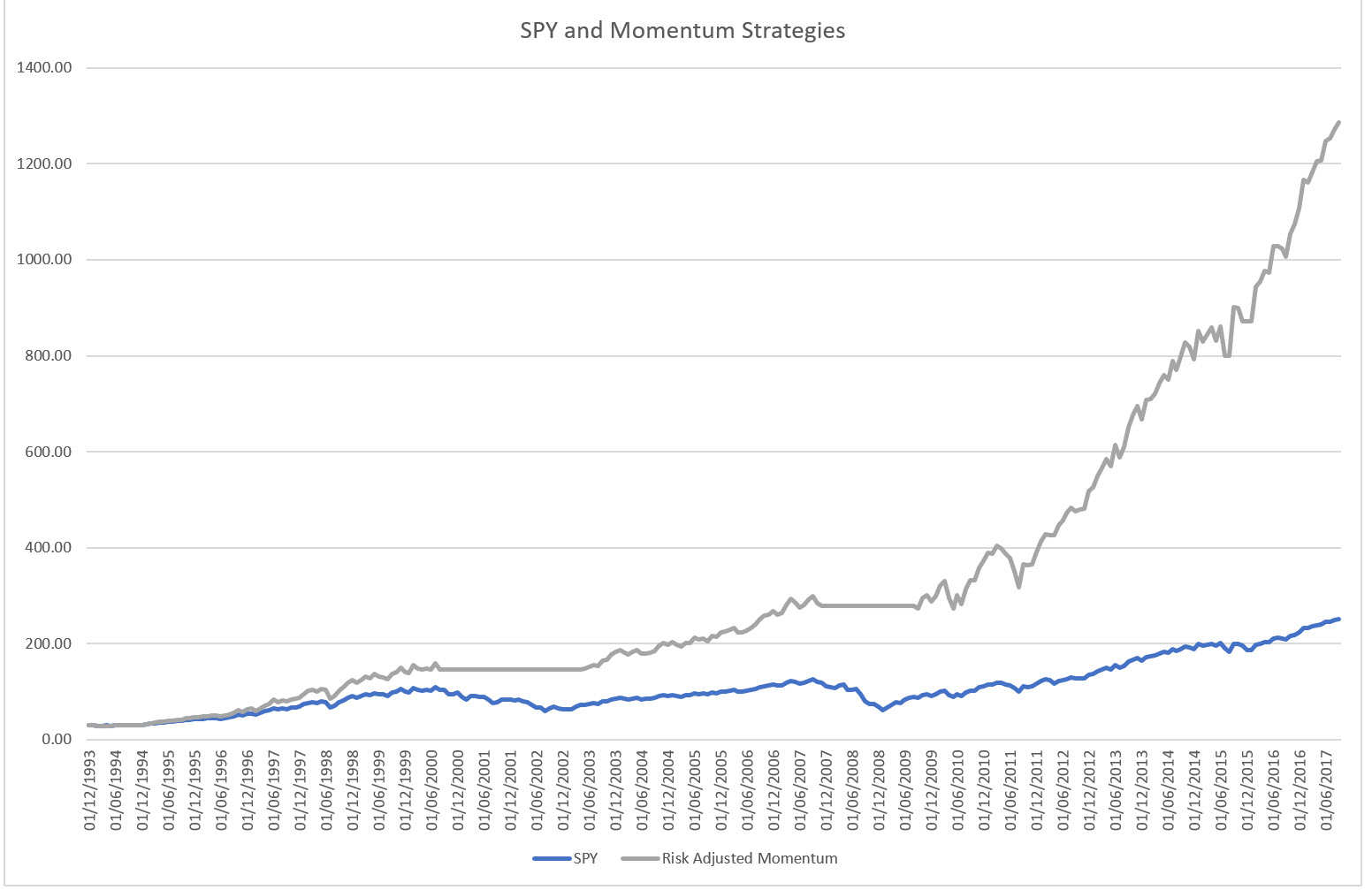
Wow!

That’s pretty impressive.

Recall what it really looked like, however:

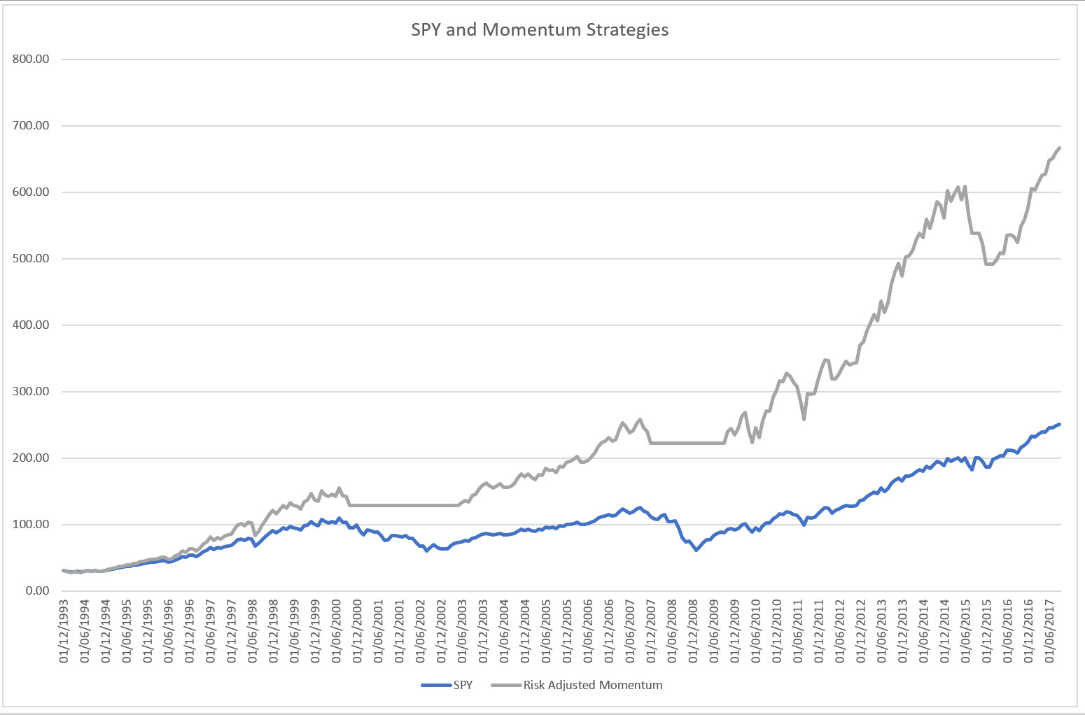
That’s a bummer.  We overstated performance by 100%!  What went wrong?

For anybody, who’s implemented anything in Excel, you’ll know how easy it is to get references mixed up.  In this particular case the Look Ahead bias entered by trading the 12^th month of our lookback period.

I.e. rather than trading the 13^th month, using the prior 12 months’ information, we traded the last month of the 12-month lookback period, even though we already used that month to form our trading decision.  It’s like assuming you have a crystal ball!

The really insidious thing here is how 12-month momentum and 1-month momentum are so strongly correlated!  You would have assumed that it wouldn’t make that much difference!

Now obviously a situation like this can only arise when you backtest.  Unfortunately, you only go live after you have a good backtesting result, and so it’s not surprising that, given a Look Ahead bias makes backtests look so nice, this error keeps on rearing its head.

Either check your tests, or forward walk your system to see that you are indeed testing realistic rules.

In-Sample Statistics

So how did we fall prey to the Look Ahead bias in the previous article, and what is our saving grace.

As was pointed out, we risk adjusted our 12-month momentum strategy.  Here it is again:

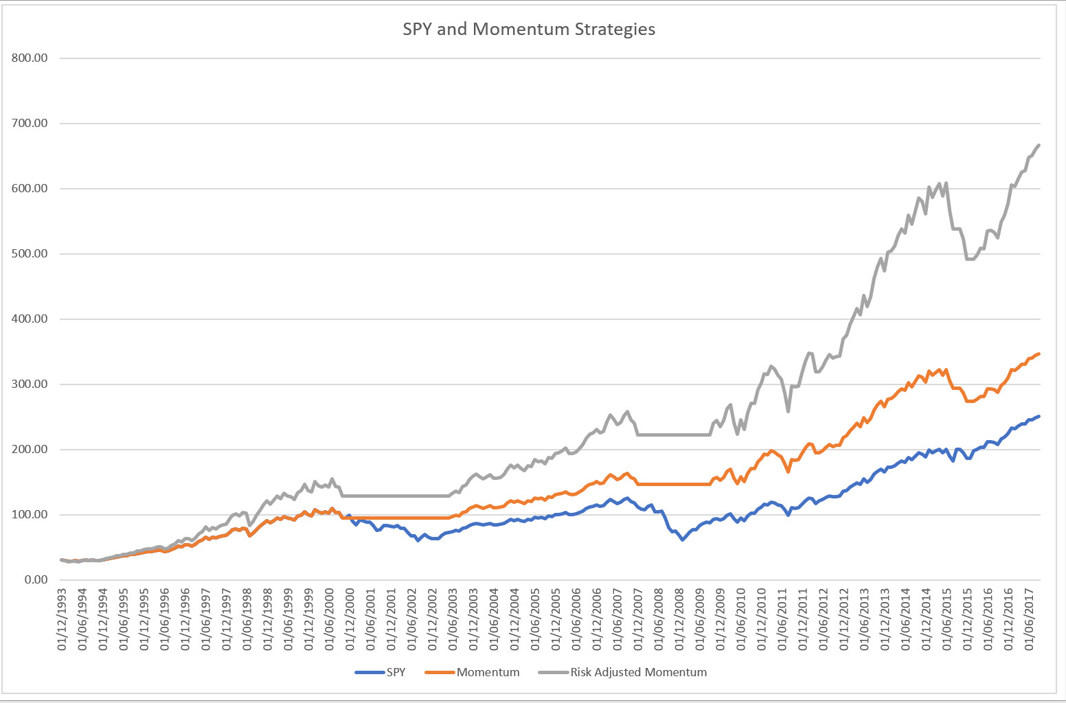
And to do that, we had to measure the risk of the S&P 500 and that of the Momentum strategy and scale up the Momentum strategy appropriately.

And if you recall from the previous article, we did that by measuring the standard deviation of both strategies.

But HANG ON!  How can we do that if in 1994, we have no clue how these strategies will pan out over the next 23 years?!

That’s where we got clonked.

The scaling factor turned out to be 1.3x, based upon these “Forward Looking” risk measures (which were nothing more than the standard deviations of the P&L streams of either strategy).

A possible solution was to use an expanding window for our risk measure.  Meaning at each time we measure the risk from that point in time all the way back to 1994 (the start of our simulated trading).

This actually ends up giving us a much lower risk multiplier, and hence a much lower performance for the risk adjusted momentum strategy.

Indeed, an issue.

Resolution

There is, however, a saving grace for us in all this, and it actually gives us even more confidence in the momentum strategy.

Our saving grace is that the stock markets didn’t just magically appear in 1994!

If you recall from the first article in this series: Building Profitable Trading Systems, we had data (albeit synthetic) going all the way back to 1871.

So, let’s try this.  Let’s estimate the relative risk from 1871 until 1994 for both the S&P 500 as well as its momentum filtered counterpart.

It so magically turns out that the relationship of 1.3x is stable!  The risks from 1871 until 1994 were nearly identical as for the period 1994 to 2017!

Now that is remarkable indeed.

It means two things:

• Our initial analysis still stands
• Going forward we can rest assured that we don’t have to fiddle too much with our risk multiplier, since it has been stable at the same value (at least to O(0.1) ) for the last 150 years.

What else does this do for us?

It underscores the stability of our approach.  Going back to gaining confidence from statistical measures, it implies that structurally markets have stayed very similar over modern times.  And this gives us confidence to proceed with this strategy.

Over-Leverage, the Second Bane

This leads nicely to the second point that was raised.

What is the optimal leverage I should use?  It turns out that simply risk-adjusting the momentum strategy does leave a lot of money on the table.

Accepted wisdom recommends using a leverage factor equal to the Kelly criterion.

This Kelly factor is usually evaluated using statistical properties of the return series.  In particular:

\( \lambda = \frac{\mu}{\sigma^2} \)

Where \(\mu\) and \(\sigma\) are the average rate of return and the standard deviation of our momentum strategy.

There are some caveats here.  Naively plugging our mean and standard deviation estimate using this formula gives an optimal leverage factor of 8.8.

This leads to:

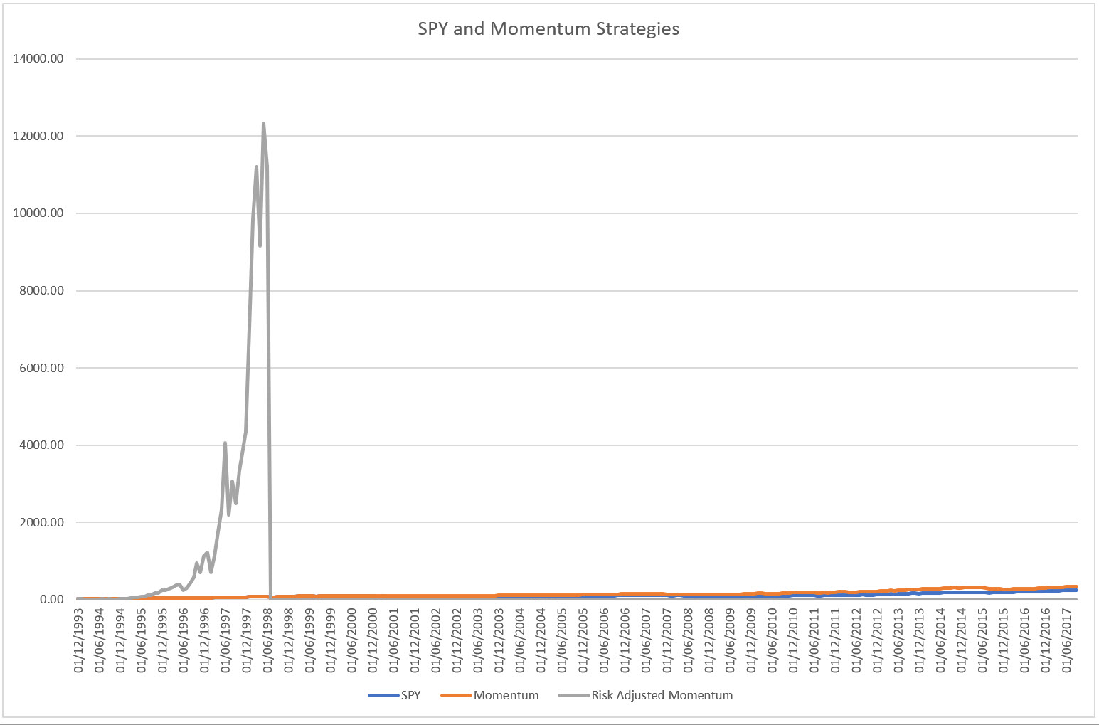
which is a cataclysmic result.

And furthermore, how on earth is this possible?

The simple answer: Over-leverage.

Let’s define Over-Leverage: the naïve assumption that we have all available, all possible, information at our disposal, and we have the over-powering desire to ride the ragged edge of disaster.

Obviously, this is a fallacious assumption and attitude.  (You’ll see towards the end how this leads to the notion of a Stop Loss).

So how could we rectify our example above?

Let’s wind the clock back a bit, and work out Kelly from first principles.

Principles:

• The returns of our asset / trading strategy are normally distributed.
• We can safely ignore any risk terms coming from higher-order moments of the normal distribution

The way these assumption feed into Kelly is visible from the structure of the formula: it only includes the mean and the standard deviation of the return distribution.

So, this leads us to the conclusion that maybe our Momentum Strategy isn’t as normal as we might assume, and might have riskier higher order moments than a normal distribution.

Let’s check this.

Kurtosis, \(\kappa=1.8\), and skweness, \(\gamma_1=-0.25\).  It’s got fat tails, which isn’t surprising for a momentum strategy, and interestingly enough a negative skew.  Now, this is interesting because on the one hand you’d expect positive skew for momentum strategies (viz. the MAN AHL article: Positive Point of Skew), however, for stocks skewness of the strategy tends to be negative (cf this great article Skewness Enhancement), indicating that you can fall off a cliff.

So how do we deal with this?

Let’s go back to the derivation of Kelly.

If our wealth process evolves like \({\displaystyle V=V_0\prod_i{(1+\lambda X_i)}}\), where \(\lambda\) is our leverage, and \(X_i\) is the return over a time period, we can find the optimal leverage, the Kelly leverage, by optimizing the expected growth rate with regards to our leverage factor.

Writing out the expected growth rate:

and taking into account that our returns are identically distributed over all time-steps (iid), we can Taylor expand \(g(\lambda)\) as:

The optimization means taking the derivative of \(g(\lambda)\) with respect to \(\lambda\), and setting it equal to zero:

In the case where we assume kurtosis and skew to be zero the Kelly-leverage \(\lambda\) ends up being our usual suspect.

However, we obtain a cubic equation if we include the higher order moments.

Thank goodness for the Italians having found solutions for this in 16^th Century (del Ferro, Tartaglia, Cardano, and Bombelli).

Working out the four moments for our case of the momentum strategy and using the algebraic solution for a cubic, we obtain an optimal leverage factor of 7.35.

Now this looks good, it’s lower than before, and it seems to have noticed our fat tails and negative skew.  But is it good enough??

NO!

We still fall off a cliff.  And I don’t even have to look at a chart.

Do you want to know why?

Because in 1998 August, the Russians went boom, and the stock market took a big nose dive.

Our momentum portfolio lost 14% that month.  And 14% x 7.35 is bigger than 100%, meaning with this leverage we would have lost it all.

What went wrong with our super-duper maths?

Simple, that event was a massive outlier.  The next biggest loss for the momentum strategy is at 7%.  This means that the kurtosis is even bigger than we estimated from our sample.

So what solutions do we have?

There are two possibilities in our case:

• We cheat! Meaning that since our strategy derives from the underlying market, why not use the skew and the kurtosis of the S&P 500?  This would allow us to benefit from the increased returns and lower volatility of the momentum strategy, but still take into account the potential for big losses from the S&P500!
• We follow the madding crowd and use half-Kelly instead.

For option (1) we obtain a leverage of 6.0, which is not too far from the optimal leverage at 6.32 (if you numerically fiddle with the numbers).  For option (2) we’d obtain 4.4.

What would the difference in performance be?  Option (1) yields a 11,800x return, and option (2) a return of 3,900x.  I would say it’s ball park similar!

Forgetting for the time being the ludicrously high numbers (not that they are ridiculous), the real question arises: even if we used the S&P 500’s fatter tails, we haven’t really guarded against a cataclysmic event in the future: we simply don’t have a crystal ball!

Coming back full circle, this is where ultimately the protective stop comes in.

Protective Stops

The message is as always, the old one: you can’t forecast the future, and hence you have to put a stop in to protect yourself.

However, here is where it gets more refined.

The stop I’m talking about is one that protects your capital from disaster.  I’m not talking trailing stops, or stops set at some arbitrary point, where a trade signal has been negated.  The cows haven’t come home yet on the subject of where the ideal trading stop is.

However, with respect to disaster recovery, it’s clear you need them.  The position depends on your risk appetite.  There are people out there who are quite happy to stomach a 90% loss.  Do you belong in that camp?

Recap

In this article we covered some foundational details of developing trading systems.  In particular, the dangers of backtesting and over-leverage:

• The Look Ahead bias can creep into your analysis in the most devious of ways. Always be on the look-out, especially if your equity curve is too much of a straight line in your tests
• Over-leverage is a killer when you least need it: in the worst-case scenario. It’s the reason places like LTCM, Amaranth, Peloton had to book the losses they did (as well as Howie Hubler at Morgan Stanley, and with him the rest of the US housing market).  So, decide a level at which you will get out, just for the sake of keeping alive (as long as it’s not at -100%!)

In addition, we had some numbers excursion that have been quite fun, and have led to some better ways of calculating the usual leverage ratios touted out there.

If you want to incorporate these, here is the extension of the previous Python code:

See You Next Time…

Next time round, we’ll be continuing with a technical variant of mean-reversion for equities which has proven profitable over the last 25 years, and which doesn’t let up. (Double promise!  No detour foreseen).  In particular, we’ll look at various ways of understanding market regimes.

I’ll also utilize our analysis on Kelly betting to give you a taster on what portfolio construction entails, and how to go about extracting as much value as you can out of your very own simple momentum / mean-reversion equity portfolio.

So, until next time,

Happy Trading.

If you have enjoyed this post follow me on Twitter and sign-up to my Newsletter for weekly updates on trading strategies and other market insights below!