
Taking Control of Your Trading Numbers – that means actually being able to replicate the results that others produce. It’s the only way to be sure that you know what’s going on.
Well, many people got back after last week’s article asking about the details of the calculations as well as about some of the more technical jargon:
- What do I mean by asset?
- What’s an asset bias?
- What does it mean to risk-adjust returns?
- How can I go about calculating the charts in the article?
- How do I actually trade this?
This is the danger with being so specialized in a topic: I tend to take the basics for granted. And hence the need for this detailed side-track.
So before jumping in to the second article in this series, Building Profitable Trading Systems Using Mean-Reversion, I felt that it would be better to cover the basics. To get you to the point where you feel you are in control of the trading numbers that are being presented online.
At the end of this article you’ll find both an Excel spreadsheet and a Python script to replicate the calculations. You’ll have a foundation for taking control of your trading numbers
JARGON BUSTING
Let’s start by busting some of the complex words:
- Asset: anything you can buy and sell and has some form of intrinsic value. An equity, a bond, maybe even a wine bottle
- Asset bias: the price of the asset has a clearly defined price pattern. Meaning that you have an edge on forecasting what will happen next.
- Edge: there’s a greater than 50-50 chance of your forecasted outcome occurring. Meaning that in the long-run your forecasts tend to work out, and hence add to your bottom line.
- ETF: stands for Exchange Trade Fund. In the previous article we focused on the SPY ETF because it allowed us to trade the S&P 500. An ETF is a fund managed by a fund manager, who specifies the strategy they will follow (e.g. track the S&P 500). The fund then issues shares which can be easily traded on the stock exchange. Over the last 20 years there has been a proliferation of such instruments tracking almost everything under the sun.
With this jargon busted let’s take a look at what we actually did in the previous article:
SIX STEPS TO TAKING CONTROL OF YOUR TRADING NUMBERS
Step 1: We chose equities as our primary asset to investigate. Why? Because we saw that they have an upside bias.A shout out to Murray who came back with a very good question: How can I tell if this is statistically significant? In other words, how do I know that I can trust this feature.
Well, for starters it’s the long-term nature of this feature that has gotten me convinced. The chart spanned 150 years! Not convinced, here is something going back 600 years:
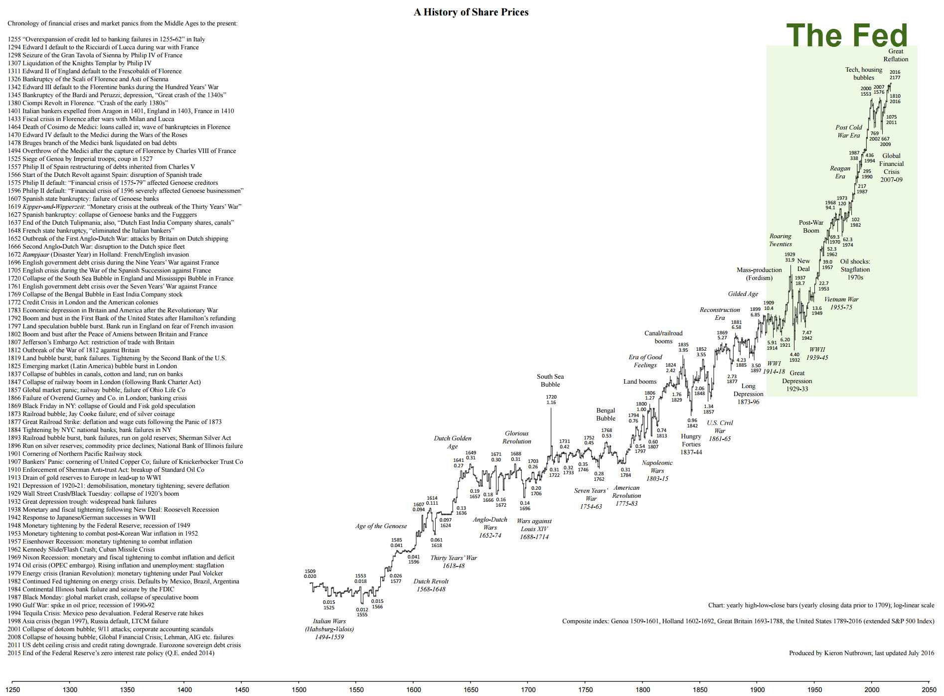
You see, from a statistical point of view, it’s not just important to have many datapoints, but to have them span a significant amount of time. Any econometrician worth his salt will rather want 100 data points over the last 100 years, rather than one million data points over the last 2 months.
Why? Because establishing that the same patterns have been around for a much longer time, gives you the confidence to say that they will persist.
And remember, the whole point of trading is to make forecasts about the future with a certain degree of confidence. For that you need an Edge. And an Edge means having a better than 50-50 chance of my forecasted outcomes occurring!
Step 2: We chose the S&P500 as a benchmark index for the equity market. There is a bit of a sleight of hand involved here. When we say equities, many people think of single stocks. The big problem here is that there are literally thousands of stocks available for us to trade.
And many of these stocks come and go. Look at Eastman Kodak. The biggest camera company in the world had to file for bankruptcy, and re-structure its business after more than 100 years. Enron, Worldcom, Northern Rock, Merrill Lynch, Lehman Brothers also fall into the category of dodo-stocks.
Do you really want to have the headaches of wondering which of your investments will be around tomorrow?
One thing we know for sure: the market will be (if it isn’t neither will you). And that’s the purpose of the S&P500: to track the market. It is an average of the 500 biggest companies in the US. If one goes bust, another takes its place, but the index is still there.
And the people responsible for managing the SPY ETF (which tracks the index) are responsible for kicking the individual shares of companies which are about to go bust out of their holdings.
By trading the market we cut all the fluff around having to worry about individual equities, and we can make macro statements about the economy instead. Something that (at least in my opinion) is easier and less time consuming.
Step 3: We chose an index which included its dividends re-invested. This is an important concept!
You see, when you own a share, that company most likely will pay out dividends back to you, as the shareholder. These dividends are part of the profits the company makes, and as a part-owner of the company you are entitled to these profits.
Now you have a choice: either blow the dividends on some fancy gadget, new home, or luxury holiday, or take that money and use it to buy more shares.
Choosing the latter option of buying more shares will give you a bigger exposure to the market, and make you more money ultimately.
That’s why we focus on the Total Return index, which measures performance with dividends re-invested! (This is the Adjusted Close in the Yahoo Finance data you can download)
Step 4: We analysed a set of rule-based strategies, so that we could compare them to the market benchmark, the S&P 500 with dividends re-invested.
The whole point was to present a set of black-and-white rules which you could follow without thinking. Remember: trade something that is tested and validated on rules which are replicable and repeatable! Otherwise you won’t have a clue what you should do in the future.
And most importantly the strategies we chose only required you trade once. I’m not sure I made this point amply clear in the previous article!
You see, a lot of trading guides will advocate screen staring, and intraday trading.
There is a really simple rule of thumb here: The amount of pain you experience grows like the square of the number of times you observe the market. This relationship has to do with the volatility of the market. Details aside, it means that observing the market twice as much, means experiencing pain four times high. You get the picture.
Therefore trading once a month puts you squarely in psychological nirvana!
Step 5: To make comparisons fair amongst the various investment options we risk-adjusted the returns. This is probably the opaquest of all technical terms used in the article, so let me dive into a bit more depth here.
Risk is defined by how much our P&L fluctuates. To be precise, if we buy an asset or follow a strategy we will be booking a P&L for every day we hold that asset. This P&L will be just the change in value from the previous day and represents our profit or loss.
We can measure this P&L in dollar terms, but this isn’t very helpful, since it doesn’t tell us how much we started out with in the first place. That’s why people use percentages. It tells you the fraction of money, given your initial investment, you would have booked on that particular day.
Equipped with this percentage P&L we can chart out a distribution of the daily returns.
Let’s do this now for the S&P 500 buy and hold strategy, where we look at monthly returns. To be clear, I define monthly returns here as the percentage returns from month-end to month-end. For instance: take the closing price in September, divide by the closing price in August and subtract 1 to get the percentage change of the S&P 500 over the month of September.
If this return is +1.0% it means that if we had started with $100 we would have ended up with $101 after the month of September. You see, working in percentages is actually a very useful approach.
By using the index which includes dividend returns we also include the effect of dividends upon our returns.
The resulting distribution of S&P 500 monthly returns is:
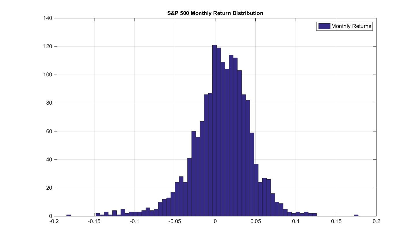
So how do we use this distribution to determine the risk of the S&P 500? Going back to the idea of risk as being encapsulated by our P&L fluctuations, we would like to know how much these fluctuations are on average. In a sense, we are looking for the average thickness in the above distribution. The technical terms is Standard Deviation (the STDEV function in EXCEL!).
For this distribution the average P&L swing is 4%. That is, 4% per month.
Now for a really important point: if I know that my P&L swings 4% a month, how much does it swing on a single day, or how much should I expect it to swing over an entire year.
Here it gets a bit tricky, because risk (or volatility as it is known) doesn’t scale linearly with time. It scales via the square-root of time. A formula is worth a thousand words:
- A year is 12 times longer than a month. So rather than taking my monthly risk of 4% and scaling it up by 12, I scale it up by the square root of 12 which is roughly equal to 3.5. So, my monthly P&L swing is roughly 14%. So I should expect the S&P 500 on average to be up or down by roughly 14% every year.
- A day is a twentieth of a month (there are 20 business days in a month). But again, it doesn’t mean that my risk for the day is a twentieth of 4%. Actually, I need to divide 4% by the square root of 20 = 4%/4.5 = 0.9% swing per day.
You see from this that volatility is not the most intuitive of concepts. At its heart it codifies the notion of randomness. And randomness bears some very unintuitive facts.
So, back to the original question: risk adjust returns?
Simple: we multiply the returns of one strategy so that its standard deviation is equal to the standard deviation of our base strategy. In this way both strategies have the same risk, according to the definition of risk we have provided above: equal average P&L swings!
Step 6: We implemented the Momentum strategy. Why Momentum as a bias?
Well, just like Equities have shown a persistent tendency to go up, momentum strategies have performed similarly.
Here is an interesting result that shows momentum applied to various assets (starting with 10 in 1300 all the way up to 90 in 2000) over the last 700 years:
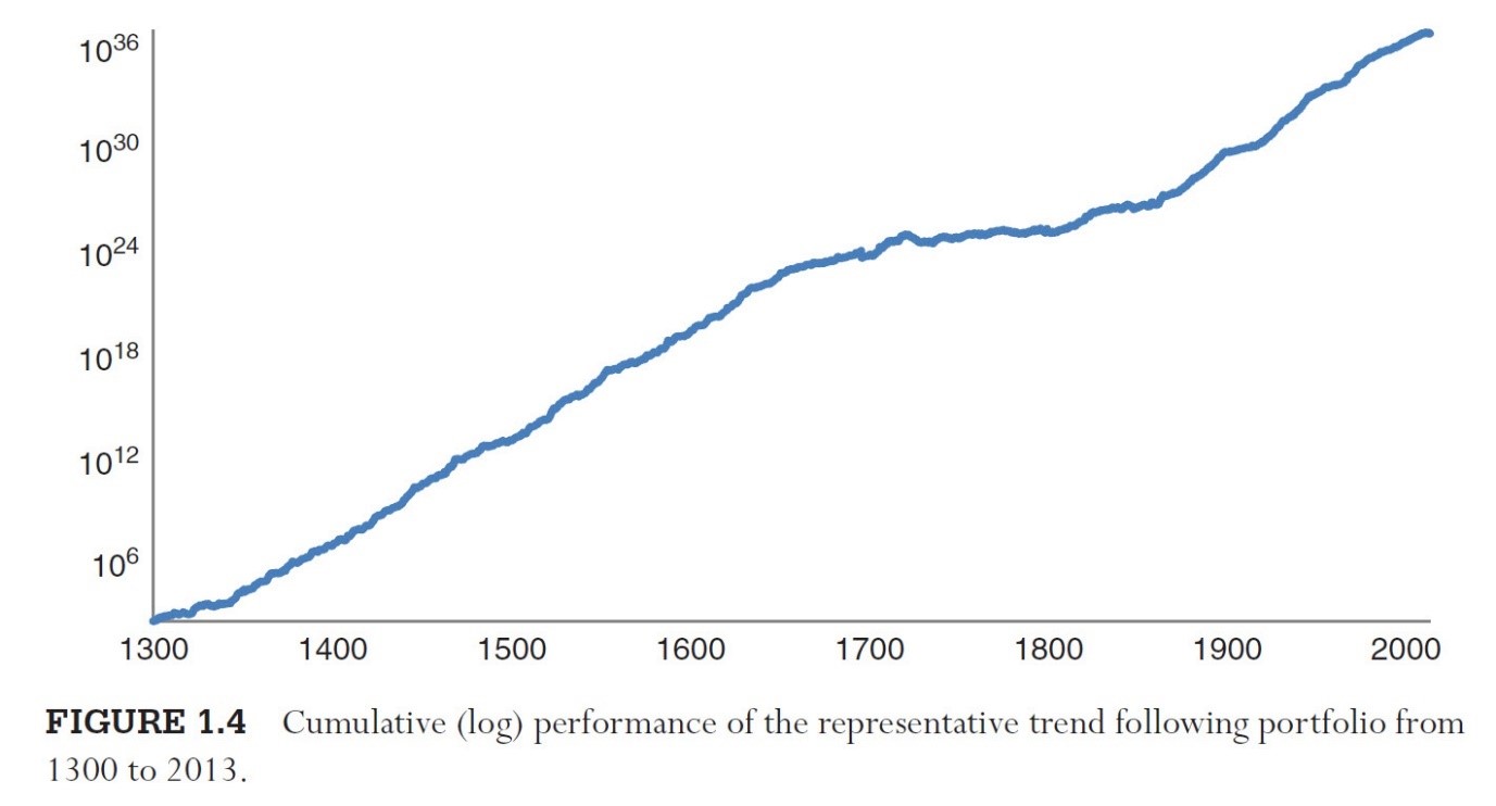
That’s a pretty impressive result!
So how did we apply this to the SPY?
In line with the philosophy of trading stress free, you observe the value of the SPY at the end of every month. If this value is bigger than the value 12 months ago, you hold the SPY. If not, you sell your holding (and put your money in a cash account earning interest).
At the end of the next month you perform the same observation. If the market has recovered and is again higher than it was 12 months ago you enter the market again.
Note: you only trade at the end of the month, and always with reference to its level 12 months ago.
Since we are focused on the Total Return performance, meaning dividends reinvested, you need to take this into account by looking at the Total Return series.
APPLYING THEORY: TAKING CONTROL OF YOUR TRADING NUMBERS
Now, this was a lot of theory to take in.
So, let’s go ahead now and actually replicate some of the charts from the previous article.
Data Sources
For starters our data source will be: SPY
Here’s a screenshot:
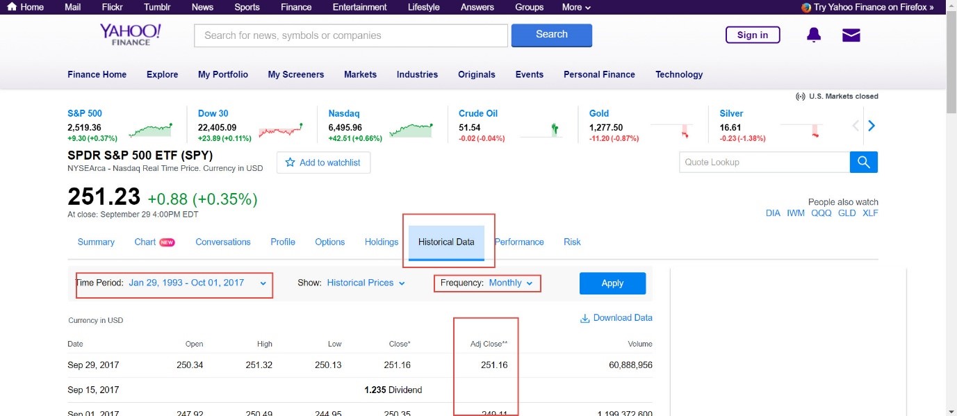
Note the areas with red rectangles. These are the fields you have to modify. And the Adj Close will be the data series we will be using, after you download the data.
Excel Backtest
Once you have downloaded the csv file, you can start applying the rules we just discussed in Excel. The spreadsheet looks like:
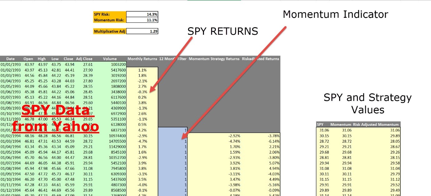
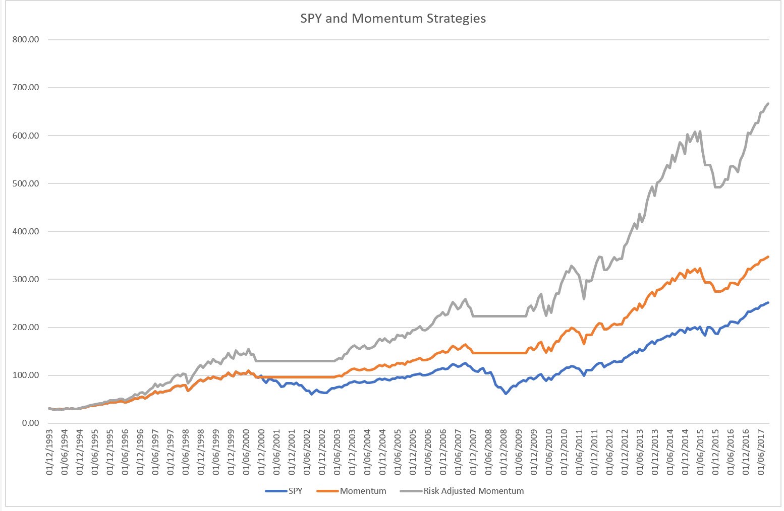
You can download the spreadsheet here, and you’ll get the chart of the risk-adjusted Momentum strategy compared to the SPY buy-and-hold strategy:[wpdm_package id=’2069′]
Python Backtest
For all you Python fanatics, here is the script in Python. You can obviously change it to apply to any ticker you want.
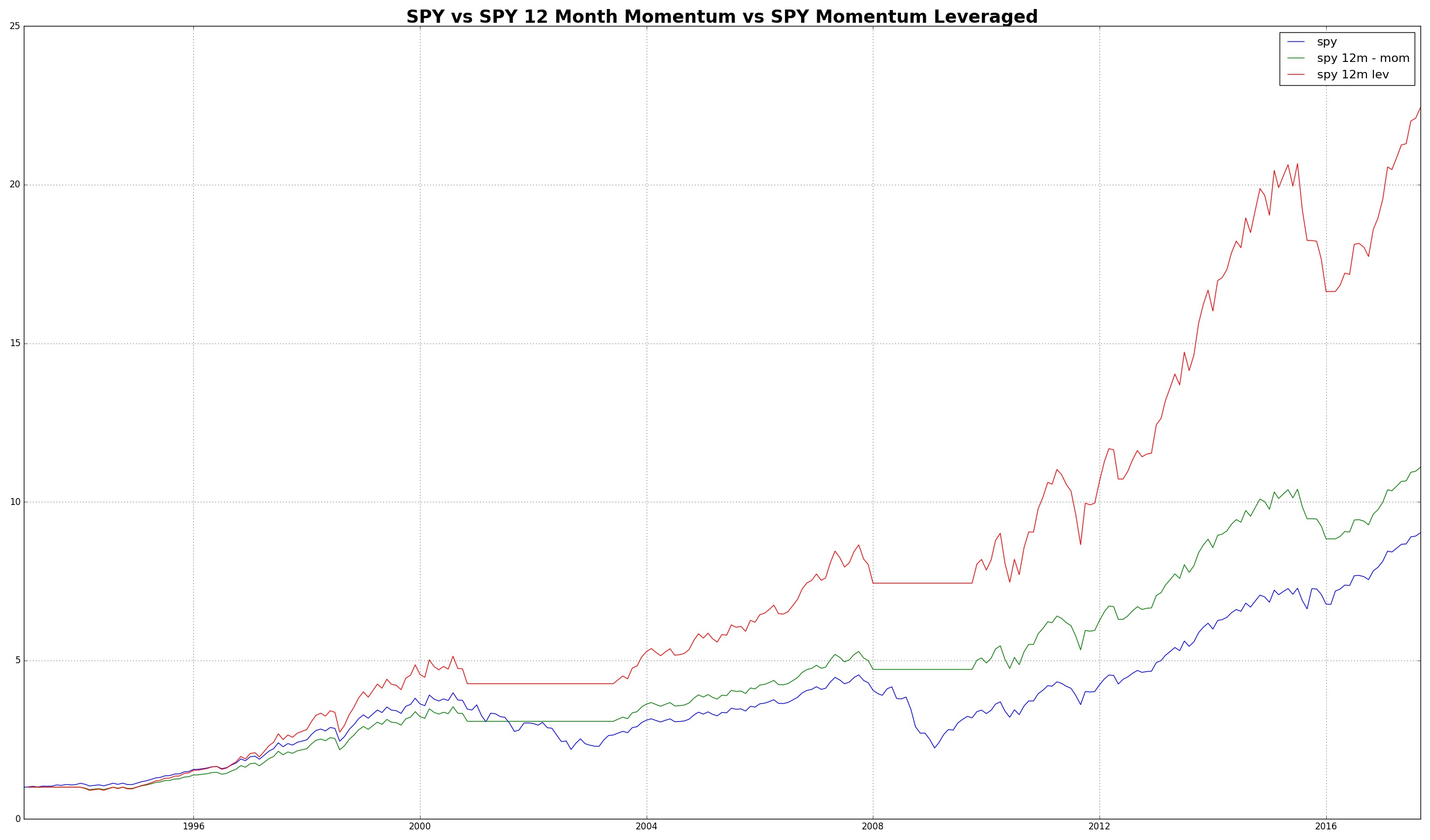
1 2 3 4 5 6 7 8 9 10 11 12 13 14 15 16 17 18 19 20 21 22 23 24 25 26 27 28 29 30 31 32 33 34 | import matplotlib.pyplot as plt import numpy as np from pandas_datareader import data as pdr import fix_yahoo_finance as yf yf.pdr_override() if __name__=="__main__": data = pdr.get_data_yahoo('SPY', start='1990-01-01', end='2017-10-02', interval="1mo") c = data[["Adj Close"]] c["spy"] = c["Adj Close"] / c.ix[0,"Adj Close"] c["rets"]=c["spy"]/c["spy"].shift(1)-1 c["flag"]=np.where(c["Adj Close"]>c["Adj Close"].shift(12),1,0) c["mom_ret"] = c["flag"].shift(1) * c["rets"] std_spy = c["rets"].std() std_mom = c["mom_ret"].std() fac = std_spy / std_mom c["mom"] = (1+c["mom_ret"]).cumprod() c["mom_lev"] = (1 + c["mom_ret"] * fac).cumprod() plt.plot(c.index, c["spy"], label="spy") plt.hold(True) plt.plot(c.index, c["mom"], label="spy 12m - mom") plt.plot(c.index, c["mom_lev"], label="spy 12m lev") plt.grid() plt.title("SPY vs SPY 12 Month Momentum vs SPY Momentum Leveraged", fontdict={'fontsize':24, 'fontweight':'bold'}) plt.legend(prop={'size':16}) plt.show() |
You’ll also have to make sure that the necessary packages are installed (as specified in the import section), however, a package manager like conda from Anaconda will make this easy for you. Also note, that you need to be using Python 3.x to make this run.
The end result looks like identical to the Excel output (however, you can now easily test this strategy by changing look back lengths, the ticker and more!):
RECAP
The purpose of this article was to get you up to speed on the details of the previous article.
We’ve covered:
- Jargon Busting, in particular what I mean by selecting Equity as and Asset which exhibits an upward bias as well as a momentum bias, and how you can trade it by using ETFs.
- I showed you why trading the market is easier than trading single stocks.
- I also hammered the point home: trade infrequently, sit on your hands. Vol scales as square root of time, and hence the more frequent you observe, the higher your experienced pain will be
- What it means to take dividends into account
- How we risk adjust returns (remember: just multiply your returns to make the risk the same!)
- And finally, how to actually trade the momentum strategy and what the underlying calculations look like.
This forms a solid foundation for the continuing articles in the series, in particular when it comes to understanding how to allocate money amongst the various components.
One thing we still haven’t covered: how does a simple multiplication of a return translate into actual position sizing at my brokerage? For that matter, what is a brokerage, and how do those guys deal with my multiplicative factor?? Don’t worry, that’s what the rest of the article series will cover!
See You Next Time…
Next time round, we’ll be continuing with a technical variant of mean-reversion for equities which has proven profitable over the last 25 years, and which doesn’t let up. (Promise! No detour foreseen)
I’ll also give you a taster on what portfolio construction entails, and how to go about extracting as much value as you can out of your very own simple momentum / mean-reversion equity portfolio.
So, until next time,
Happy Trading.
If you have enjoyed this post follow me on Twitter and sign-up to my Newsletter for weekly updates on trading strategies and other market insights below!

Hi Corvin!
excellent article! as usual!
regarding the risk adjusted returns: there is a look ahead bias there
it is calculating the std() on the whole series , at time t, we don’t now the std at time t+1
one option is to use a rolling window on the std() or an expanding window:
std_spy_exp=c[“rets”].expanding().std()
std_mom_exp = c[“mom_ret”].expanding().std()
fac_exp=std_spy_exp/std_mom_exp
c[“mom_lev_exp”] = (1 + c[“mom_ret”] * fac_exp).cumprod()
it compounds to 15 instead of 22 times the initial capital, still good
what about kelly optimal_f? I tried :
kel=c[“mom_ret”].mean()/c[“mom_ret”].std()**2
c[“mom_lev_kel”] = (1 + c[“mom_ret”] * kel).cumprod()
seems to blow? have you tried kelly on this?
Hi Peter!
Thank you very much for your comment!
You are absolutely right 🙂 There is look-ahead bias involved here in determining the standard deviation, and you’re expanding() amendment fixes that. And you are completely right on the Kelly criterion.
On the former, try this: plot out the ratio of the standard deviations on the expanding window. The ratio has a very nice smooth behaviour, stabilizing ultimately around 1.3.
The reduction in performance you observe is derived from the fact due to the uptrend from 1993 onwards, both the Momentum Strategy and the SPY are long. This means that one inherits the volatility of the other, and the ratio is pegged to 1.0, hence there is no amplification of returns. Post 2001, the expanding window ratio quickly stabilizes to 1.3, which is the long term ratio. This is due to the crash in the SPY in 2000/01 which is avoided by the Momentum Strategy, and hence the two standard deviations diverge from each other.
So here is an interesting question: what would happen if we were to estimate the long-term ratio by using the equity data going back to 1871 (from the previous article)? I’ll do the calcs, and post the result here.
Ex-ante (haven’t done the calculation yet), I’d expect this behaviour to be stable enough, that leading into 1993, from 1871, we get a stable ratio of 1.3, ultimately replicating the above behaviour (yes, yes, I’m justifying myself a bit here!). But this is just a guess. Quite exciting to do a backward looking out-of-sample test!
On the Kelly Criterion, you have to be careful. The assumptions going into the formula you are using is that returns are normally distributed (i.e. no skew, and not fat-tailed), and no auto-correlation. In our case that is not the case. I.e. we have a first big outlier of -14.1 percent in September 1998, due to the Russian default, which would have wiped out a Kelly leveraged investor (at 8 times), since 100/14.1 < 8. Why? Because Kelly overestimates leverage for financial distributions!
The article series is naturally leading up to that.
And to give a bit of a teaser, assuming zero auto-correlation on the return series of your portfolio returns, there a is a nice relationship between the time to doubling of your wealth and the Kelly criterion.
This is how I feel the Kelly criterion and derivatives thereof should be employed: time estimates of potential return targets. I feel that people tend to overlook time in their trading completely, though it is a constant factor influencing their behaviour. Restlessness and boredom leads to over-trading, feeding the blinking lights on your trading screen.
People are so focused on return distributions without taking time into account, that they forget Keynes’ quote: “In the long run we are all dead.”
Hi Corvin
many thanks for your answer, looking forward to your updates!
very good point about the non-normally of returns leading to kelly blow ups
is the volatility adjusted factor your preferred position sizing method? or do you have others?
another option would be half-kelly, on a expanding window or rolling window, doesn’t blow (assumes it can go short the Mom Long strat)
kel_half=c[“mom_ret”].expanding().mean()/c[“mom_ret”].expanding().std()**2*0.5
c[“mom_lev_kel_half_exp”] = (1 + c[“mom_ret”] * kel_half).cumprod()
it compounds to 63343 times initial capital (with nerve wrecking drawdowns, that’s for sure 🙂 )
would be great if in this series you could also discuss your approach on portfolio construction: how an investor could combine multiple strategies in a portfolio:
if you have momentum, carry, PPP, etc…given the correlations between these strategies
Hi Peter!
Just realized, that the calculation for the long-term standard deviation is in the first article in the series: Building Consistently Profitable Trading Systems.
The long term vol for the S&P 500 is 14% (going back to 1871 … granted it is an artifical index prior to the 1950s), and the filtered momentum series is at 10%. This is pretty much in line with the sample stats for 1993 until now (which is actually quite remarkable).
Caclulating the sample stats only up to 1993 (the start of the SPY backtest), gives very similar numbers. I’ll put the numbers up in the next article.
In essence, recent history is a reflection of what’s happened over the last 100 years and more!
With regards to portfolio construction, that’s exactly where I’m heading towards. Though your comment chain has side-tracked me, and the next up-coming article will be with regards to skew/kurtosis correction for Kelly, as well as some stats properties regarding the S&P 500 market. I find the stability very interesting.
However, as of next week it’ll be back on track.
ok thanks Corvin! looking forward to your updates!