Equities Mean Reversion and Market Regimes

In this second part of the Mean-Reversion in Equities series we’ll cover the reasons behind why mean reversion works in various market regimes.

In the previous article we combined the idea of looking at two consecutive down-days combined with buying the S&P 500 while it was below its five day moving average.

A question that stands out: why does it work so well? And, will it ever stop?

The answer to this question lies at the heart of developing good trading strategies.

Table of Contents

What’s a Trading Strategy?

Ultimately a trading strategy is a procedure that generates buy/sell signals from the information made available to it.

The underlying assumption therefore is that markets are driven by the factors we are trying to exploit.

So a trading strategy ultimately means determining the factors that drive the market, determining how strong they are and if they are persistent. And then finding a way of overcoming the market noise to get the most value out of our trades.

Some well-known factors are: momentum, mean-reversion, economic fundamentals.

You’ll probably be familiar with the fact that choppy markets are anathema to trend-following.

And of course overly trendy markets are bad for mean-reversion.

Economically motivated strategies such as macro strategies assume that markets over time converge to some economically implied value for the asset.

But how can we determine if the factors we wish to trade are actually present?

For the purpose of this article series, as in the previous articles, we’ll focus on the S&P 500 whilst answering these questions.

Market Regimes in Equities

How can we detect market regimes? Usually the simplest methods tend to be best.

The ones we want to focus on in this article are mean-reversion and by association, momentum; one being the mirror image of the other.

The way we usually understand mean-reversion is as a tendency to move counter to the direction of the most recent moves. Usually off the back of an overextension.

Momentum on the other hand is nothing more than a continuation move.

So what would be a really naïve strategy to exploit either of these behaviours?

In the case of mean-reversion we can simply trade in the opposite direction to yesterday’s move:

\(\mathrm{\mathrm{Position}}_{today}=-\mathrm{sign}(\mathrm{Return}_{\mathrm{yesterday}})\)

In the case of momentum we revert the sign on the right as we are trading in the direction of yesterday’s move

Not that difficult!

So let’s check it, as far back as we can.

Market Regimes in the Dow Jones Industrial Index and the S&P 500

The two data series most easily accessible and going back far enough are the Dow Jones Industrial Index going back to 1900 and the S&P 500 for which we can easily obtain data back to 1950. Both of these sources have daily closing data.

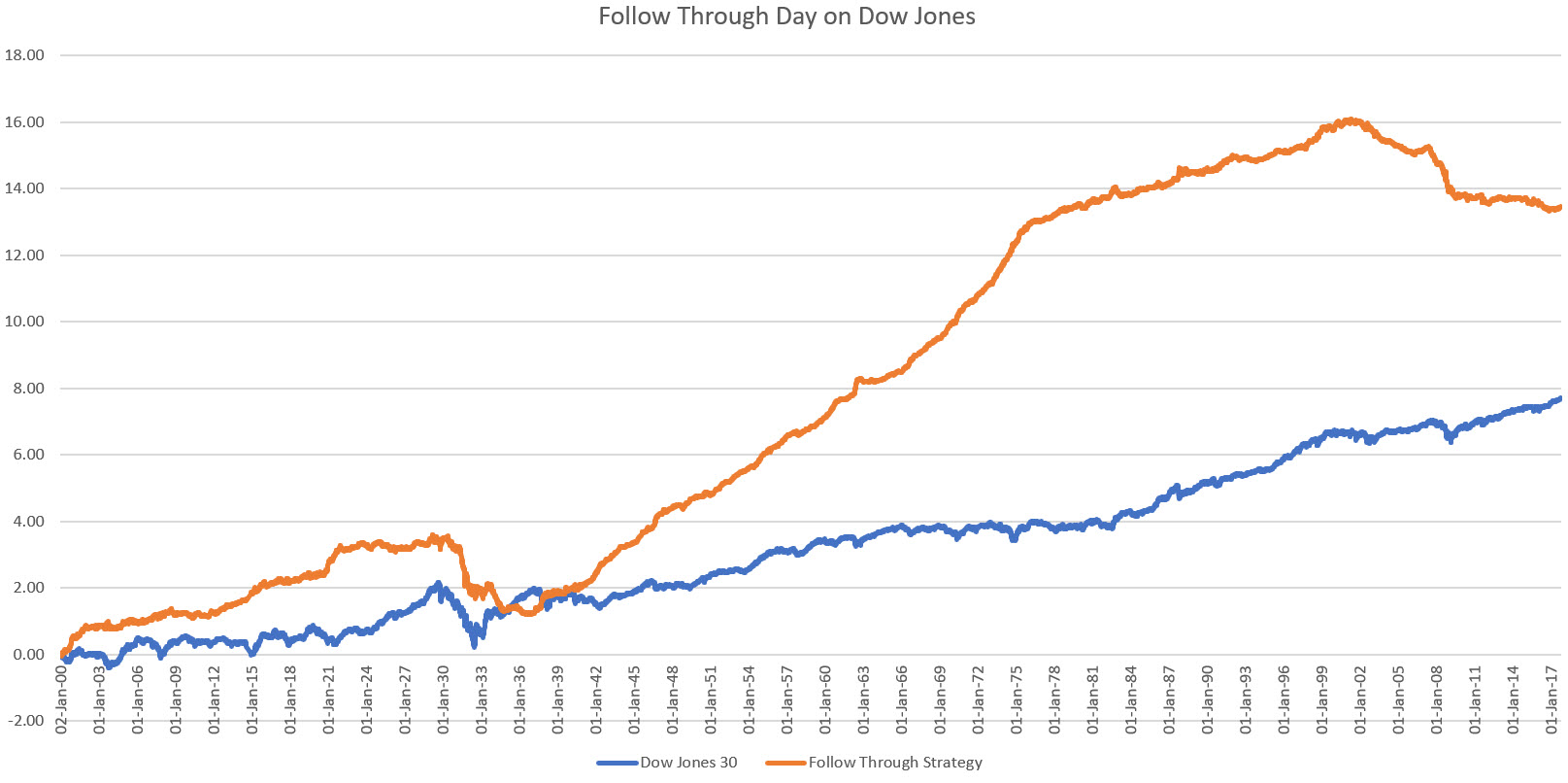
Applying the momentum strategy to both these indices we obtain (where we are treating returns as additive):

and

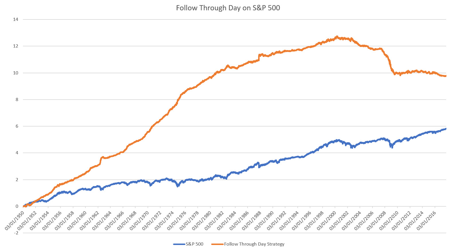
Both these charts exhibit some very fascinating and consistent behaviour (which is the reason we chose to focus on momentum first, rather than run the mean-reversion counterpart).

Most of the time we spent in a trending market. You can see this by the incredible performance of this naïve strategy. (Note: we haven’t taken any commission / slippage into account here!)

There were times when the trendiness switched sides, and we became strongly mean-reverting (as can be seen in the loss making periods of this naïve momentum strategy).

These periods coincided with the post-1929 era and the post-2000 era. Both experienced big crashes.

So, how does that influence our expectations about mean reversion?

To answer this question let’s apply the two systems we described in the previous article to both these indices and see how they performed.

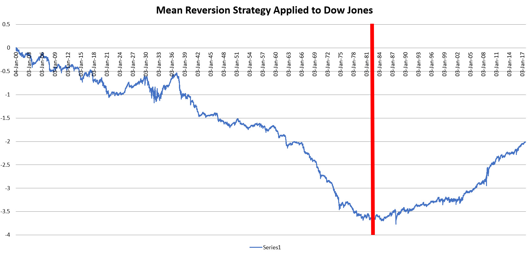
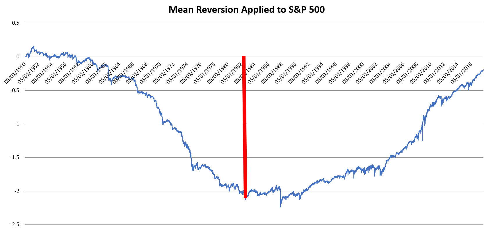
Mean Reversion Strategy Applied to Dow Jones

We see that prior to 1982, the performance was actually a straight line down.

So mean-reversion beware! Even if the bonanza has lasted the last 35 years, over the real long-term it didn’t fare too well!

Measuring Market Regimes in Equities

As we saw, the P&L on naïve strategies is quite an efficient way of establishing the regime we are in.

Is there another way?

Yes: Autocorrelation. Autocorrelation measures the tendency of a market to follow through on the previous day’s move. In excel we simply use the CORREL function where the input is the same return series, but offset by one cell from itself.

Let’s apply the 1-day autocorrelation (using the past year’s data) on the S&P 500 return since 1950 and overlay a two year moving average on top of it to smooth out the oscillations:

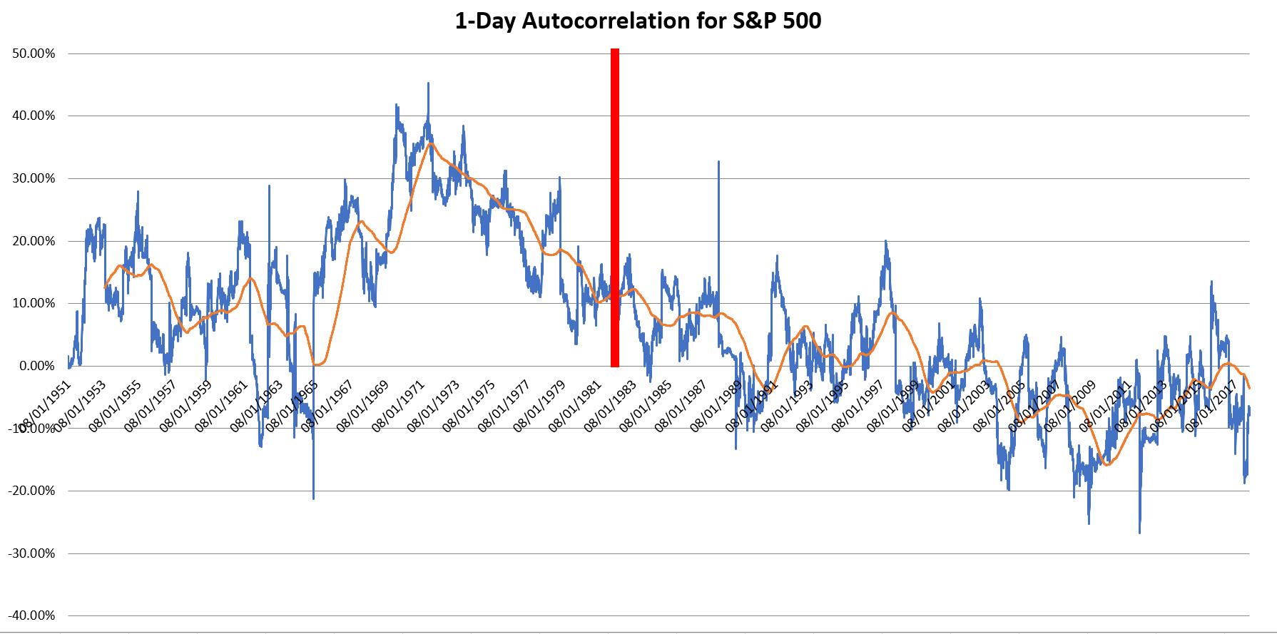
We have been firmly in a mean-reverting regime since the early 80s, as can be seen from the autocorrelation starting to poke below zero and then firmly staying in that territory.

Many things could have changed the market dynamic; one thing that does stand out is that S&P 500 futures started trading in 1982 on the CME, though I admit this might a tenuous relationship (for instance no index futures were introduced shortly after the 1929 crash).

Another explanation might be that the shocks markets experience during significant crashes tend to drive a change in behaviour of market participants from trendiness to mean-reversion.

Meta-Trading Regimes

It is always relevant to understand the market regime you are in.

The regime will ultimately determine the kind of strategy you can apply.

For instance post 2013 EURUSD intraday ranges collapsed, and intraday strategies were at a big disadvantage.

In the case above we can see that mean-reversion did not work well in trending markets.

It’s therefore not just necessary to design indicators that have some form of predictive power. It’s more important to understand the underlying statistical tools you can use to obtain information about the characteristics of the market. As well as the properties of these measures.

In essence you are building a market scanner, that will be able to tell you which strategies to apply.

What’s highly interesting in the case of the equity market analysis above, is the persistence of the underlying behaviour, be it mean-reversion or momentum. We are talking decades.

Simulating Markets (For the Technically Minded)

A good systematic trader (aka market scientist) also works the other way. Once he thinks he has found a statistical feature that provides juice he creates a lab. In our particular case it would be great to see if the autocorrelation feature is the true driver behind our 2 down day system.

All we need to do is create a time series that has those features. In essence a controlled version of out S&P 500 index.

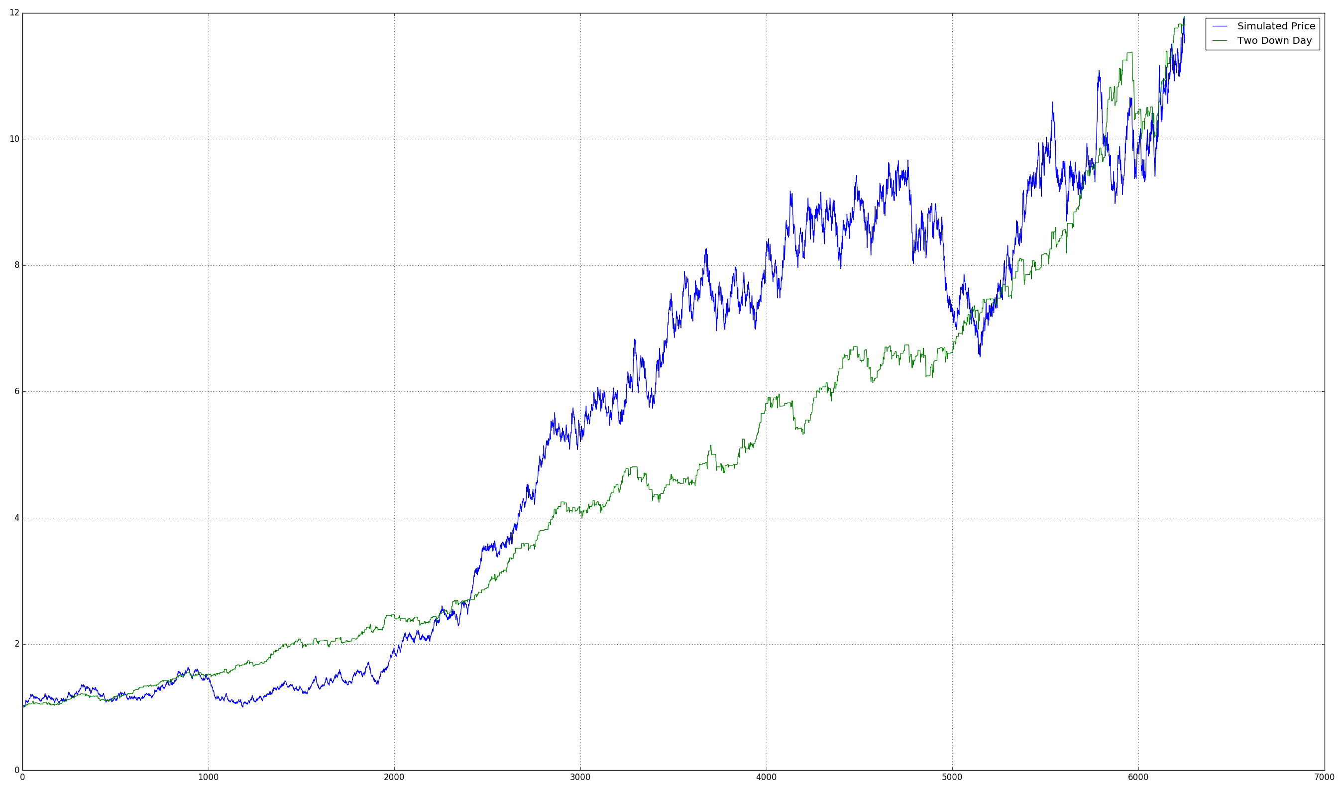
Below is the Python code to do this. The parameters we are using are estimated from the S&P 500. We generate the autocorrelation by simulating an AR(1) process from gaussian random variables. Here is a result from a sample:

1
2
3
4
5
6
7
8
9
10
11
12
13
14
15
16
17
18
19
20
21
22
23
24

import pandas as pd
import numpy as np
import matplotlib.pyplot as plt

r = np.random.normal(0.0, 1.0, 6250)

ac1 = -0.064
ac2 = -0.00453

mu = 0.0003515
std = 0.011385
df = pd.DataFrame({'rand': r})

df['rand_ac'] = df['rand'] + ac1 * df['rand'].shift(1) # + ac2 * df['rand'].shift(2) # --- uncomment
df['ret_sim'] = mu + std * df['rand_ac']
df['px'] = (1 + df['ret_sim']).cumprod()

df['sig'] = (df['ret_sim'] < 0) & (df['ret_sim'].shift(1) < 0)
df['sys'] = (1+df['sig'].shift(1) * df['ret_sim']).cumprod()

plt.plot(df.index, df['px'], hold=False, label='Simulated Price')
plt.plot(df.index, df['sys'], hold=True, label='Two Down Day')
plt.grid()
plt.legend()

[Note: to keep the article from over-running I’ve cheated here. A two down day strategy really requires an AR(2) process. And indeed if you work out the autocorrelation lagged by two days for the S&P 500 you see exactly that. Uncomment the code to run these controlled experiments. And if you’re up to it, check out that the down 2 day actually doesn’t do that well for a simple AR(1) process! Autocorrelation is more subtle than meets the eye!]

As expected the P&L is driven by the statistical feature we baked into the model.

Currency Markets

In currency mean-reversion is slightly more subtle. Using the pattern based approach (i.e. the 2 down day) is not necessarily the best method of extracting value. There is a lot of underlying noise in the currency pairs.

However, the 5-day moving average acts as a great smoother.

You also have to find the right pond to fish in. USDJPY is an explosive pair and even to this day quite trendy.

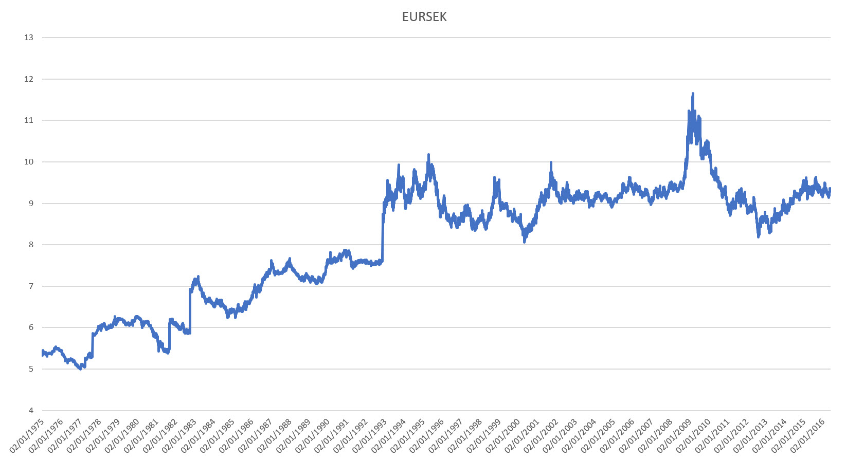
A great mean-reverting pair is EURSEK. Have a look at the long term chart:

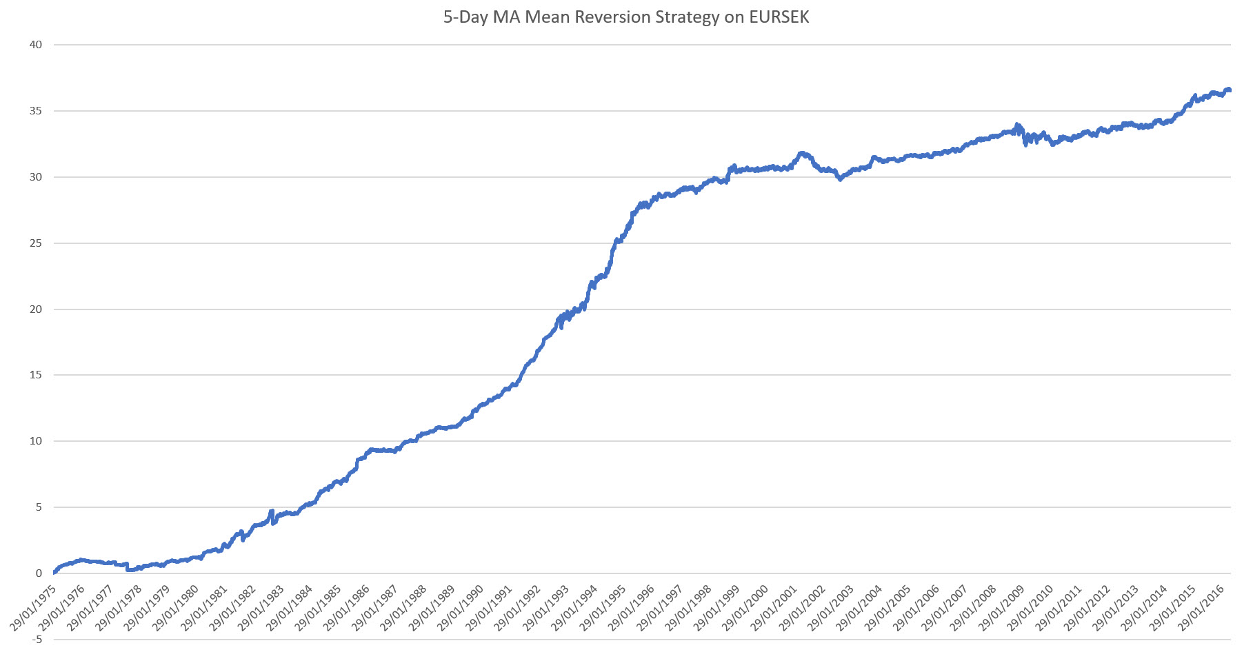
And applying the 5-day moving average approach from the previous article produces following result:

Recap

This article addressed the concerns as well as the criticisms that are levelled at the types of mean-reversion strategies we have been looking at:

They haven’t always worked
They’re over fit

In actuality the systems are so simple, that the second can’t really be levelled at them. The first point however is valid: and a long back test shows that they didn’t always work.

But that’s the point of the saying “the only constant thing about markets is that markets will always change.”

You have to understand what drives your system to ensure that it will continue to function. If the underlying cause changes or disappears, so will your system.

Here we identified a statistical feature of the equity market that does contribute to the performance as we saw from our “lab” experiments.

See You Next Time…

Today’s article acted as a general disclaimer: these systems work; now. They didn’t always work, but, we’ve done our darndest to nail down when they might fail and how to detect if the market conditions are right.

With this setup we are ready to move on to a twist on the mean-reversion combination we’ve been covering. And then add to that the Equity momentum strategies. That’ll be portfolio composition for you!

So, until next time,

Happy Trading.

If you have enjoyed this post follow me on Twitter and sign-up to my Newsletter for weekly updates on trading strategies and other market insights below!