
Of all things on this planet?! Aren’t they boring? Not explosive enough? Isn’t this stuff what old people invest in? Also, aren’t they supposed to start to sell-off? And how do you get your hands on these over the counter instruments.
In the first article of this series on Creating Profitable Trading Strategies we started with the premise that you need to look at assets and their underlying biases.
We covered equities. They’re exciting. Buffett makes 19.1% a year on them. And as we’ve just seen in the last month, they provide us with some great roller-coaster rides.
Not only that, they also exhibit some nice consistent long-term behavior such as long-term momentum and short term mean reversion.
As far as equity indices and a simple approach we’ve squeezed the lemon sufficiently.
Let’s move on the next vegetable (uh fruit): Bonds!
Intro to Bonds
So, what’s a Bond. Before you invest in a Bond you got to know what it’ll give.
A government bond (which is what we’ll focus on in this article), is a piece of paper issued by a government which is the equivalent of an IOU. And just like when you borrow from a bank, the government has to pay back this loan.
The first ever general bonds were issued by the Netherlands in 1517 (though the Netherlands didn’t officially exist, it was the city of Amsterdam). The first bonds to be issued by a national government was in 1694 by the Bank of England to fund its war against France. Up until the 20th Century many of these bonds were perpetual, in that governments did not have to repay the principal. This stopped in the 20th Century, and nowadays most bonds come with a maturity date upon which the full amount is repaid (hopefully).
The Great Things About Bonds
The great thing about government bonds is that it’s one borrower, a very big one, borrowing across lots of time frames. Why is this great? For following reasons:
Governments need to fund stuff. Like the roads we use, the hospitals we go to, and the schools we send our school children too. As well, as the armed forces that protect the country, and the police that keep us safe.
Just like most normal families, the government just can’t seem to get its act together and tends to need more money than it has. So, the government goes out and borrows. From you, the citizen of the government.
Given the funding needs, it will do so with loans of different maturities. Like your car loan, which might be only for 5 years. Your mortgage might be for 25 years. Similarly, the government needs stopgap funding, or longer-term funding to meet longer-term liabilities, or even to fix the low rates at present.
So, in essence by analysing a country’s bond market we end up being able to observe what the market is willing to lend to the government and at what cost.
And since these loans are made a wide range of maturities it can tell us some very interesting information as to what the market believes rates and the economy might do. It informs us of certain underlying expectations.
Jargon Busting
The IOU the government gives you to evidence your lending is called a Bond. The regular repayments are called Coupons (initially bonds came as certificates of ownership with paper coupons attached we you exchanged for payment, hence the name).
Now you don’t have to hold on to these IOU pieces of paper. You can sell them on in a secondary market, if you don’t want to wait for repayment, since you see another opportunity on the horizon.
Or you could buy a bucket load, since it looks like the government is actually getting out of the doldrums, and this IOU is therefore quite valuable. I.e. you’re engaging in purchasing distressed debt.
In either case you can buy and sell this IOU from the market.
Disregarding the mechanics of how this market works, how governments actually issue debt, the fact that this bond has a price is ultimately all that counts.
So, what does this price depend on?
Well, we’ve identified the three factors:
- Time left until the loan matures
- The interest rate on the loan
- And the creditworthiness of the government
Let’s assume for the sake of this article that (3) isn’t that relevant. So all we have left is time and interest.
Maths with Bonds
As you probably recall from middle school math class, if you have two variables you can plot them out.
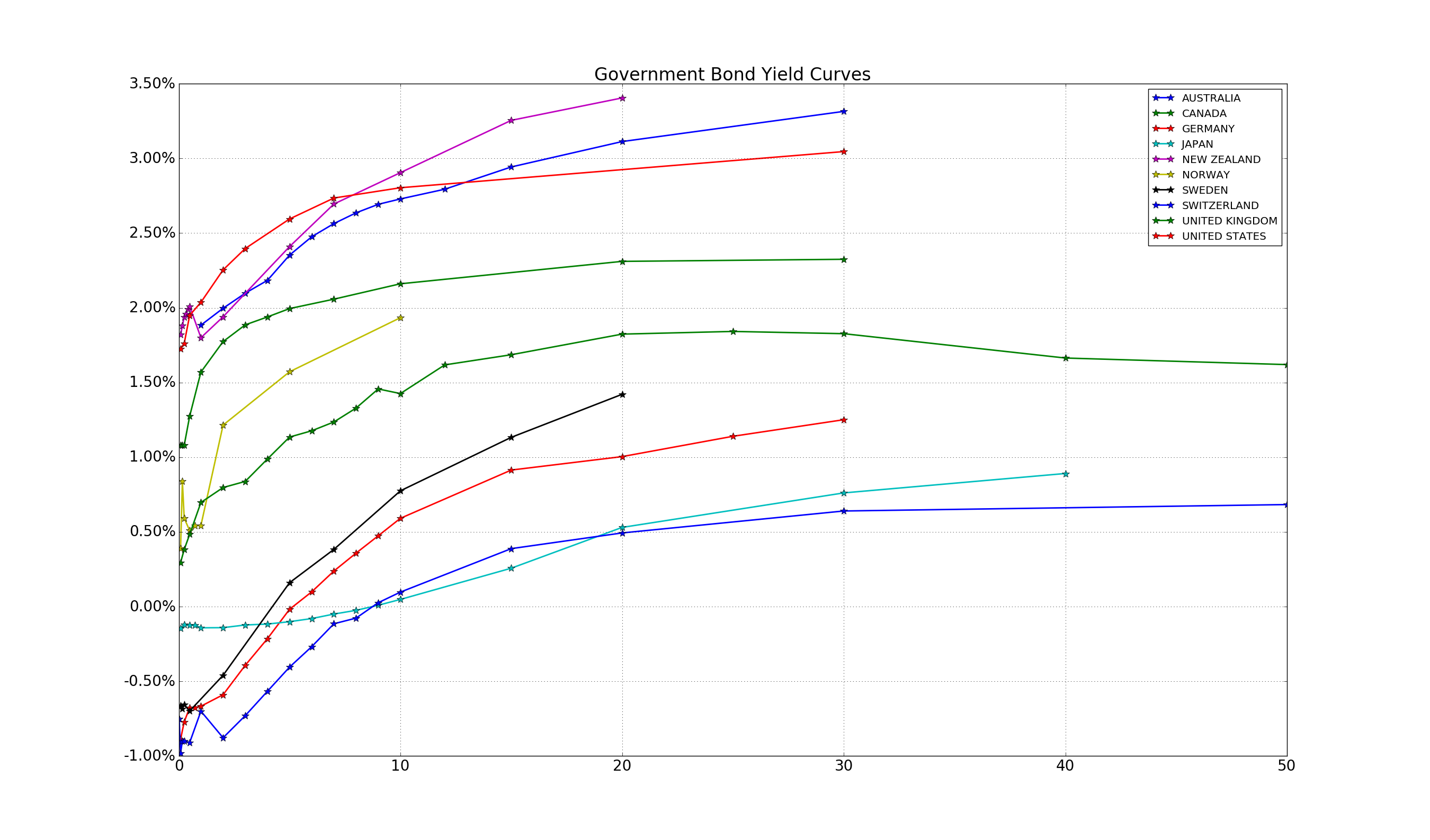
Let’s do that. Interest charged on a bond, versus time left until the bond matures.
You can find the python code at the end of this article.
The very first thing that is striking about this chart and shows the interesting times we still live in: the number of government bond yields which are negative. On the short-dated side, it shows you Central Bank policy, trying to incentive money flow, and hence increase inflation again, implicitly getting the economy up and running. By the 10-year mark rates are now close at or above zero. It shows how investors over the last two years have been willing to give up a coupon payment, in return for holding safe assets, especially during the 2016 Brexit vote. And rates are positive all round on the long-dated side.
Complex Bond Yield Curve Dynamics
The second thing you should notice is that this is just a snapshot of TODAY.
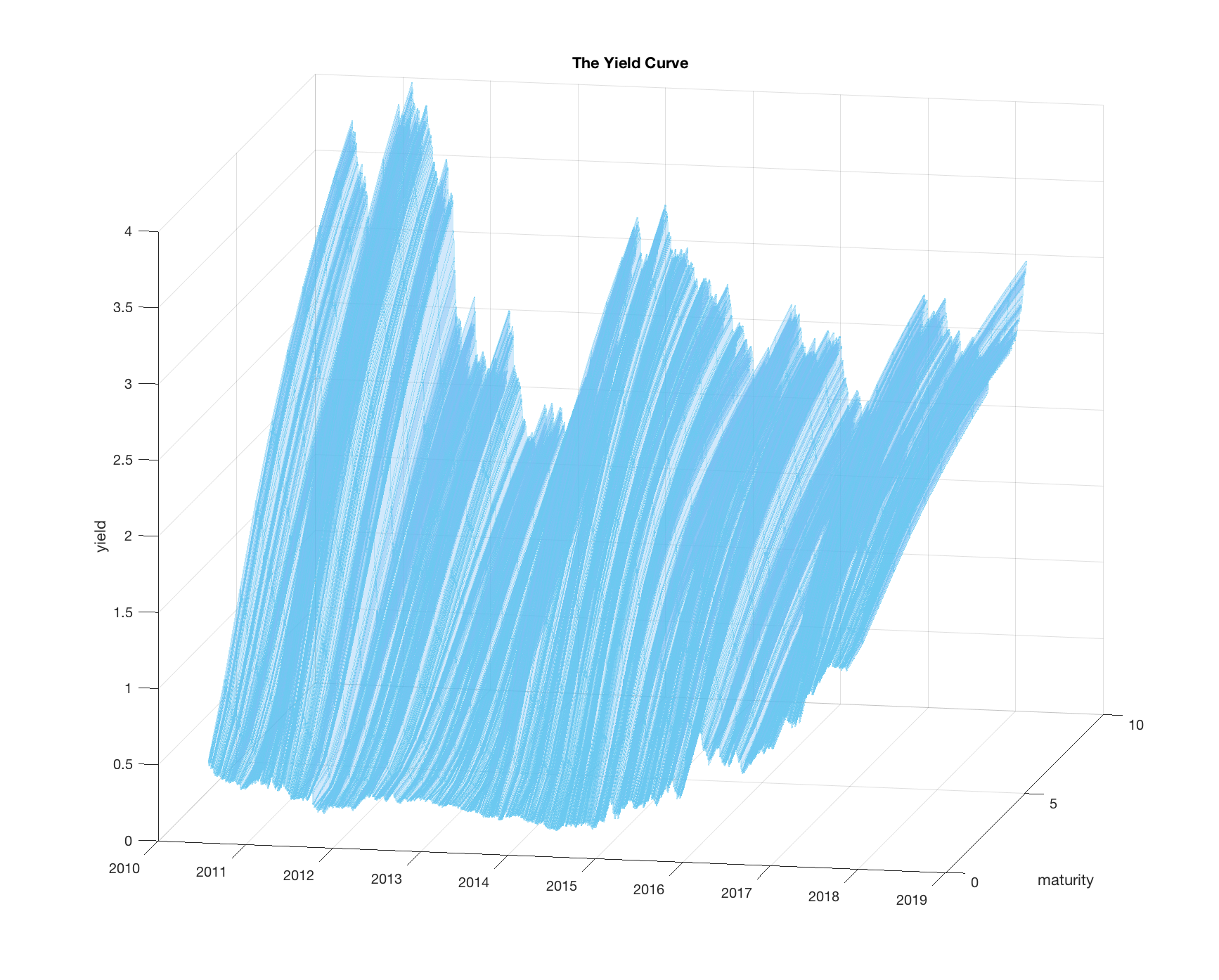
So, how would you plot a yield curve’s evolution through time?
As you can see, getting your head around the Yield Curve and how it moves through time, is much more complex than looking at the price-chart of a stock!
Rather than looking at a point moving through time, tracing out a line, you are looking at a line moving through time, tracing out a surface.
But that’s not all!
Remember that these Bonds have a finite maturity!
So, as you move through time the nature of the bonds change as well.
Let’s say you start out today with a government bond that matures in 10 years, i.e. the government pays you in 10 years’ time the full amount back, plus some interest on the way there.
Well in 1 years’ time this bond has just become a 9-year bond. Now let’s say the government wants to issue some more loans also maturing in 9 years’ time. Obviously, they have to have some relationship to the 10-year bond which now has become a 9-year bond, since both types of bonds represent the same concept: a 9-year loan.
So, you have a yield curve moving through time, and at the same time the bonds on the yield curve roll along the yield curve with decreasing maturity.
That’s a lot of dynamics. That’s why fixed-income derivative traders tend to look at FX and Equity traders as if they just got out of their caves.
Quick Summary
So, let’s have a quick summary of the bond market:
You have a yield curve
Each point on today’s yield curve represents an interest rate at which the government can borrow from YOU (that’s what your tax is used for).
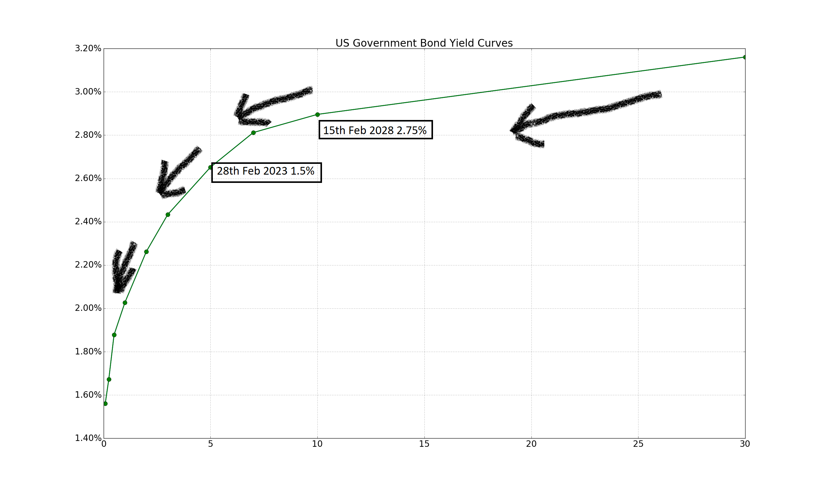
At each maturity point on the curve you have bonds which will mature at that time. As time passes bonds roll down the curve (down, because the interest rate tends to get lower the shorter the maturity).
Take a break. The following picture summarizes this:
So What?? Investing and Trading Bonds
… you might be asking. Who cares??
Well, let’s bring over our typical financial advisors.
One of the popular allocations of assets in the 80s and assets was the 60/40 portfolio. I.e. stick 60% of your capital in Equities and 40% in Bonds. Bonds were supposed to buffer you from the volatility of stocks, however, you still wanted the stock upside, since you needed the growth. Hence the 60% there.
There was also a more general rule of thumb: take your age and stick that into bonds, and 100 – your age and stick that into equities. Obviously the older you get, the more you need the income that bonds generate, rather than the growth equities provide.
In any case bonds should be added to your portfolio (how much? we’ll cover that later).
Does that make any sense?
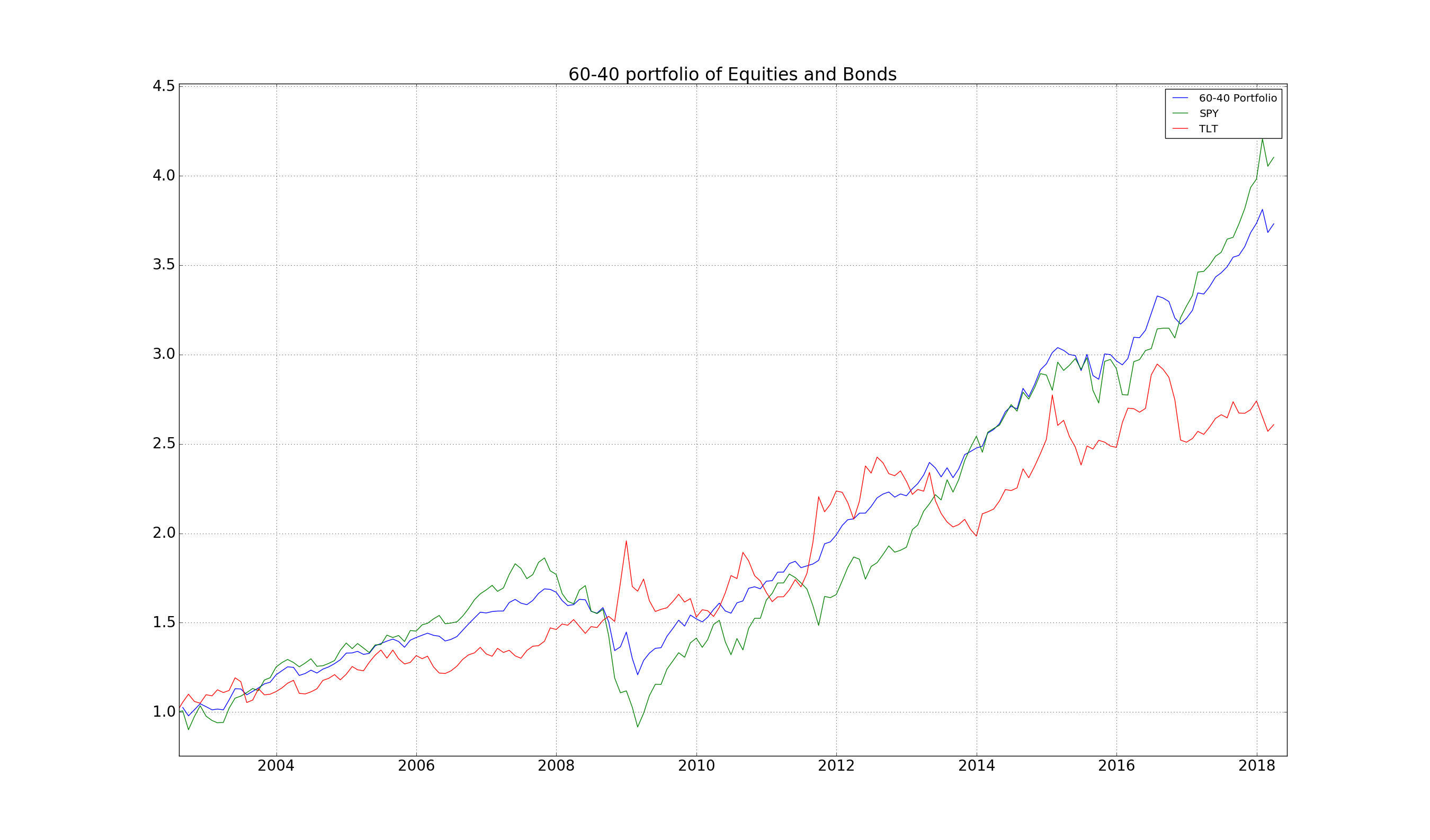
Let’s take a look. The first question to hit us: what do we use to invest in bonds? Here’s the great thing that’s happened over the last 15 years. The introduction of ETFs which track round about anything. So we can actually use the IEF which tracks 10 year US government bonds. For equities we will use the SPY which tracks the S&P 500.
And we have following performance statistics for this portfolio for leverage 1x:
| 60 / 40 | SPY | TLT | |
|---|---|---|---|
| Ann. Return | 8.8% | 10.2% | 6.9% |
| Ann. Vol | 8.3% | 14.1% | 13.0% |
| Ann. Sharpe | 1.1 | 0.7 | 0.5 |
| Max D/D | -28.4% | -50.7% | -21.8% |
So, adding bonds to our equities does indeed work out: the Sharpe Ratio is a significant 1.1, which is pretty astounding!
60/40 Portfolio
Hang on you will say, what bonds, and if they mature how do I reinvest, and do I need a PO box to get the coupon?
The great thing is that ETFs take care of all of that. They magically roll any matured bonds into new positions, and the coupons magically appear in your account for you to re-invest.
An example is the IEF from before, which looks only at bonds with maturities between 7 and 10 years.
This means that when the bonds the ETF holds start to shorten in time, their maturity becomes smaller than 7 years, they get sold and the newest batch of 10-year bonds get acquired by the managers of this ETF.
So, looking at the IEF is in essence like holding a bond that always has a fixed maturity of roughly 10 years. Or in other words, you are tracking the 10-year interest rate. In jargon, you are holding on to a constant maturity bond of roughly 10 years.
Choosing the IEF is a bit random. Do we have any other bonds to play with?
Yes, here is a list:
- AGG: iShares Barclays Aggregate Bond Fund, tracks the total U.S. investment-grade market
- GOVT: iShares US Treasury Bond ETF
- SHY: iShares 1 – 3 Yr US Treasury Bonds
- IEI: iShares 3 – 7 Yr US Treasury Bonds
- IEF: iShares 7 – 10 Yr US Treasury Bonds
- TLH: iShares 10 – 20 Yr US Treasury Bonds
- TLT: iShares 20 – 30 Yr US Treasury Bonds
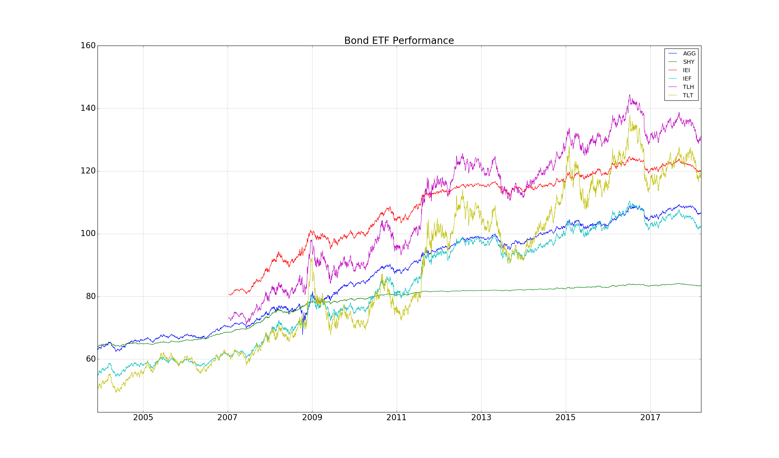
And of course it’s always interesting to see how they’ve behaved in tandem:
A simple visual inspection should indicate that selecting combinations of these bonds might actually improve the performance results we obtained above.
Quick Recap
In this post we moved on to the next asset class Bonds, and asked: how do you invest in Bonds?
These instruments are tricky, since they are finite maturity, mature and disappear. However, by utilizing tracking ETFs we can get a handle on them.
And we’ve also seen how adding them to a portfolio of stocks we can definitely improve our overall performance. Historically the Sharpe ratio has moved up to 1.1!
That is impressive behavior.
See you Next Time
Of course, there are several unanswered questions that immediately crop up:
- Given that interest rates are about to rise, can we still count on bonds to provide the performance they have?
- Instead of just being naively long stocks, what about including the portfolios we built earlier in the series?
- Instead of trading bond ETFs (or even Stock ETFs), can you trade futures? This is an interesting question, since ETFs incur a series of costs, which futures don’t. Also, futures allow for a greater leverage, which ETFs don’t, since they are classified as shares.
The next couple of articles will address exactly that! So until next time,
Happy Trading!
Addendum: Python Codes
Below is the Python code used to generate the data in this article. You can run them as standalone scripts (though you might have to ensure that you have have installed the relevant modules, such as pandas). Also, the version of Python used is 3.
Python script to plot out G-10 Government Yield Curves
1 2 3 4 5 6 7 8 9 10 11 12 13 14 15 16 17 18 19 20 21 22 23 24 25 26 27 28 29 30 31 32 33 34 35 36 37 38 39 40 41 42 43 44 45 46 47 48 49 50 51 52 53 54 55 56 57 58 59 60 61 62 63 64 65 66 67 68 69 70 71 72 73 74 75 76 77 78 79 80 81 82 83 84 85 86 87 88 89 90 91 92 93 94 95 96 97 98 99 100 101 102 103 104 105 106 107 108 109 110 111 112 113 114 115 116 117 118 119 120 121 122 123 124 125 126 127 128 129 130 131 132 133 134 135 136 137 138 139 140 141 142 143 144 145 146 147 148 149 150 151 152 153 154 155 156 157 158 159 160 161 | # Script to plot government yield curves from Investing.com # Third pary modules required: bs4, lxml, matplotlib, requests from bs4 import BeautifulSoup import requests import matplotlib.pyplot as plt INVST_LINK = 'https://www.investing.com/rates-bonds/world-government-bonds' HEADER = 'Mozilla/5.0 (Windows NT 6.1; Win64; x64) AppleWebKit/537.36 (KHTML, like Gecko) ' \ 'Chrome/64.0.3282.186 Safari/537.36' def get_inv_page(): ''' Obtain the parsed Investing.com page with the government bond yields The header is required, otherwise Investing.com will return a 404 :return: bs4 container for html ''' base_url = INVST_LINK header = HEADER pg = requests.get(base_url, headers={'user-agent': header}, verify=False) soup = BeautifulSoup(pg.text, 'lxml') return soup def get_ctry_tbls(soup): ''' :param soup: the bs4 containing the Investing.com page :return: returns the tables containing the bond data in html format ''' cts = soup.find_all('h3') tbls = [] for c in cts: a = c condition = True while condition: a = a.next_sibling if a.name == 'table': condition = False tbls.append([c.text.upper(), a]) return tbls def get_ctrys(tbls): ''' :param tbls: the list of tables from Investing.com :return: a list of countries ''' ctrys = [] for i in tbls: ctrys.append(i[0]) return ctrys def get_tbl(t): ''' :param t: an html table :return: a python list of lists containing strings ''' data = [] rws = t.find_all('tr') for rw in rws: cols = rw.find_all('td') cols = [ele.text.strip() for ele in cols] cols = [ele for ele in cols if ele != ''] if len(cols) != 0: data.append(cols) return data def get_yld_tbl(ctry: str, tbls): ''' :param ctry: the country name :param tbls: the list of tables from Investing.com :return: a html table ''' tbl_tag = list(filter(lambda x: x[0] == ctry.upper(), tbls))[0][1] tbl = get_tbl(tbl_tag) return tbl def parse_time(tms): ''' :param tms: relative time, e.g. 1D, 4W, 6M, 2Y :return: relative time as float ''' tm = tms.split(' ')[-1] if tm == 'Overnight': return 1/365.0 if tm[-1] == 'W': return float(tm[:-1])*7/365.0 if tm[-1] == 'M': return float(tm[:-1])*30/365.0 if tm[-1] == 'Y': return float(tm[:-1]) print(tm) raise RuntimeError('Time not Parsed!') def parse_ylds(ys): ''' :param ys: a python list of lists conversion from html table with string entries :return: maturity and yield values ''' tm = [] y = [] for rw in ys: tm.append(parse_time(rw[0])) y.append(float(rw[1])/100.0) return tm, y def process_all(): ''' Function which retrieves Investing.com data and returns a list of yield tables :return: yield tables ''' soup = get_inv_page() ts = get_ctry_tbls(soup) ctrys = get_ctrys(ts) ctry_ylds = [] for ctry in ctrys: y_s = get_yld_tbl(ctry, ts) tm, yld = parse_ylds(y_s) ctry_ylds.append([tm, yld, ctry]) return ctry_ylds def plot_yld(ctrys): ''' Plots yield tables :param ctrys: a list of yield tables ''' fig = plt.figure() ax = fig.add_subplot(1, 1, 1) fig.hold(True) for c in ctrys: ax.plot(c[0], c[1], label=c[2], linewidth=2.0, linestyle='-', marker='*', markersize=10) vals = ax.get_yticks() ax.set_yticklabels(['{:3.2f}%'.format(x * 100) for x in vals]) ax.tick_params(labelsize=20) plt.legend() plt.grid() plt.title('Government Bond Yield Curves', fontsize=24) plt.show() if __name__ == '__main__': res = process_all() r = list(filter( lambda x: x[2] in ['GERMANY', 'UNITED KINGDOM', 'UNITED STATES', 'AUSTRALIA', 'NEW ZEALAND', 'JAPAN', 'CANADA', 'NORWAY', 'SWEDEN', 'SWITZERLAND'], res)) plot_yld(r) |
Python script to create a 60-40 portfolio of stocks and bonds.
1 2 3 4 5 6 7 8 9 10 11 12 13 14 15 16 17 18 19 20 21 22 23 24 25 26 27 28 29 30 31 32 33 34 35 36 37 38 39 40 41 42 43 44 45 46 47 48 49 50 51 52 53 54 55 56 57 58 59 60 61 62 63 64 65 66 67 68 69 70 71 72 73 74 75 76 77 78 79 80 81 82 83 84 85 86 87 88 89 90 91 92 93 94 95 96 97 98 99 100 101 102 103 104 105 106 107 108 109 | import math import pandas as pd import matplotlib.pyplot as plt import datetime as dt from pandas_datareader import data as pdr import fix_yahoo_finance as yf yf.pdr_override() # 'AGG' # total bonds # 'GOVT' # total treasury # 'SHY' # 1-3 yrs # 'IEI' # 3-7 yrs # 'TLH' # 10-20 yrs # 'TLT' # > 20 yrs bondlist = ['AGG', 'SHY', 'IEI', 'IEF', 'TLH', 'TLT'] def get_symbol(sym): return pdr.get_data_yahoo(sym, start='1990-01-01', end=dt.date.today().strftime('%Y-%m-%d'))#, interval='d') def resample(df, freq='W-FRI'): res = pd.DataFrame() res['Open'] = df['Open'].resample(freq).first() res['High'] = df['High'].resample(freq).max() res['Low'] = df['Low'].resample(freq).min() res['Close'] = df['Close'].resample(freq).last() res['Adj Close'] = df['Adj Close'].resample(freq).last() return res def transform_monthly(spy, bond, bond_name): spy_r = resample(spy,freq='M') bond_r = resample(bond,freq='M') spyc = spy_r[["Adj Close"]] bondc = bond_r[['Adj Close']] spyc.rename(columns={'Adj Close': 'SPY'}, inplace=True) bondc.rename(columns={'Adj Close': bond_name}, inplace=True) res = spyc.join(bondc, how='outer') ix = res[bond_name].first_valid_index() res[bond_name] = res[bond_name]/res[bond_name][ix] res['SPY'] = res['SPY']/res['SPY'][ix] return res def maxdd(x: pd.Series): m = (x / x.expanding().max() - 1).min() return m def performance_stats(x, nm): ret = x.mean() * 12 vol = x.std() * math.sqrt(12) print(nm + ' return: ', ret) print(nm + ' vol: ', vol) print(nm + ' Sharpe Ratio: ', ret/vol) print(nm + ' max d/d: ', maxdd((1+x).cumprod())) def plot6040(bond='tlt'): spy = get_symbol('SPY') bond_d = get_symbol(bond) res = transform_monthly(spy, bond_d, bond) rets = res/res.shift(1) - 1 portfolio = pd.DataFrame() portfolio_rets = (0.4*rets[bond] + 0.6*rets['SPY']) portfolio['Portfolio'] = (1+portfolio_rets).cumprod() plt.hold(True) plt.plot(portfolio.index, portfolio['Portfolio'], label='60-40 Portfolio') plt.plot(res.index, res.SPY, label='SPY') plt.plot(res.index, res[bond], label=bond) performance_stats(rets[bond], bond) performance_stats(rets['SPY'], 'SPY') performance_stats(portfolio_rets, 'Portfolio') plt.tick_params(labelsize=20) plt.title('60-40 portfolio of Equities and Bonds', fontsize=24) plt.legend() plt.grid() plt.show() def plot_all_bonds(): plt.hold(True) for bnd in bondlist: b = get_symbol(bnd) plt.plot(b.index, b['Adj Close'], label=bnd) plt.title('Bond ETF Performance', fontsize=24) plt.tick_params(labelsize=20) plt.legend() plt.grid() plt.show() if __name__ == "__main__": plot6040(bond='tlt') # plot_all_bonds() |



Hi Corvin, this is an excellent article. I have never come across a fixed income trading article that summarizes the complexity in this space so well and intuitive. Out of interests, what are the strategies out there (in rising or falling interest rates environment) that traders use to trade this market and how does convexity enter into the picture? So far, I know all these fixed income concepts from my degree and terms like yield curve (normal, inverted, flat) convexity, duration, YTM, maturity but I’m struggling to translate all of these into a coherent explanation that outlines a sensible trading strategy.
Hi Gabriel,
Thank you very much for your comment!
Many of the strategies are difficult to implement for retail, since they involve OTC instruments, and shorting some of these bonds isn’t the easiest in the world. Moving over to futures, then is a different story, though many people here focus on shorter time horizons.
The main point of the article was to show that including a bond allocation in your portfolio can dampen drawdowns (which as is always my philosophy, can allow you to increase leverage!)
The real question is by how much to allocate to these instruments, other than the usual 60-40 you see banded about.
The issue here is a lack of price data. Futures go back to the 80s, and ETFs to the early 2000s. Both time periods are during a strong bull market, where you didn’t just earn coupon, but also price appreciation. So this could well be out of the norm. This is what I want to show in the upcoming article: how to go ahead and get an estimate of future price performance of bonds, should we enter the bond bear market as many forecast.
Ok thanks for the reply. I understand that there is the risk parity alternative to the 60-40 portfolio which puts more weights on bonds and enable his fund to leverage more since the returns would be unspectacular otherwise (I’m sorry to kill the suspense if this topic is the intention for your next post). Ray Dalio champions this idea and to his credit, his fund has performed well on the back of this portfolio allocation. However, maybe this could be a coincidence since we have seen a bond rally for quite some time now? I would like to have your view on this and if you agree with my assessment, is there any other “hot” alternative?
Hi Gabriel,
Risk parity certainly plays a role. It isn’t the newest of concepts, and is a method most traders employ to allocate capital, since risk based allocation, has always made more sense. Dalio has attached his name to it, however, it’s been known and implemented for way longer. The interesting thing is to think about how bond markets, and a potential uptake in yields will affect bond returns. The answer isn’t that obvious, and there are some interesting analyses that can be done, which certainly is the upcoming topic.
Regarding to hot-stuff: G10 yield curves are flat. Any bet on curvature in decent size, since you’ll need the leverage to extract value at these low rates, is what to look for. However, trading this from a retail side, with the limited instruments available is difficult.
Thanks man! I’m looking forward to your next post … hopefully I don’t have to wait long for it 😛