
Equities mean-reversion works right now.
And as part of Building Consistently Profitable Trading Systems it forms a key component.
In this article we’ll present the final version of the mean-reversion system to form part of the trading toolbox, and the final portfolio.
It’s the Larry Connor’s RSI2 strategy. And it’s based on the two concepts we covered in Equities and Their Mean Reversion Habits:
- Looking for a series of down days
- Looking for reversion towards a short dated moving average
And as we said in previous articles, the twist we’ll add is by introducing Welles Wilder’s RSI indicator.
Recall that in Building Consistently Profitable Trading Systems the stated aim was to re-use well known systems that have worked in the past and keep on working. Re-inventing the wheel can be a waste of time.
The point of trading is to exercise discipline and really intervene when systems start to behave differently from their historic norm.
With that said let’s proceed.
System Recap
From Equities and Their Mean Reversion Habits we saw that by combining two systems we obtained a solid performance. The first system required you to buy after two-down days in the SPY (the S&P 500 ETF). The second system required you to go long the SPY while you were below the 5 day moving average. Here is a P&L chart to refresh your memory:
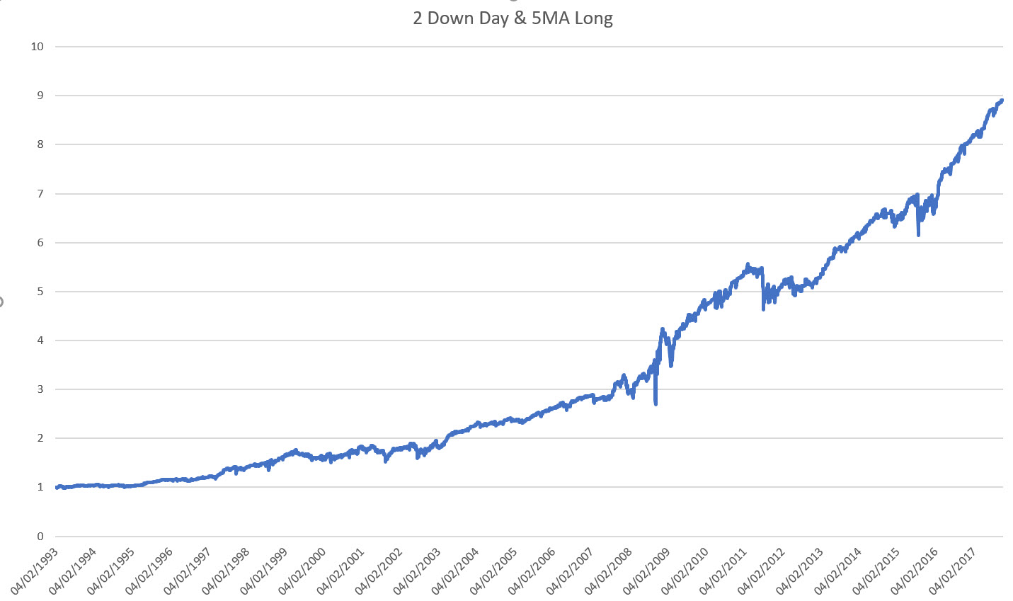
We’ll add modifications to this system and boost the Sharpe ratio it had from 0.7 to close to 1.
The primary modification is to move away from a binary signal (two down days in a row) to a continuous signal, by utilizing Wilder’s Relative Strength Indicator (RSI).
What is the RSI?
The RSI indicator measures the strength between upward and downward moves in an asset. The logic goes that if there has been a strong move in one direction then we’re due for a correction in the opposite direction.
The actual calculation looks at the average of the upward moves versus the average of the downward moves via the relative strength (where we are looking at the sizes of the moves, ignoring their signs):
\(RS = \frac{\mathrm{Avg}(up moves)}{\mathrm{Avg}(down moves)}\)
Obviously this calculation is bounded below by zero, but unbounded above.
So Wilder created the RSI which simply caps the indicator at 100 on the upside:
\(RSI=100 – \frac{100}{(1+RS)}\)
The logic goes: as you have persistent up moves, the Relative Strength (RS) becomes large, and the RSI goes to 100. If you have persistent down moves, the RS goes to zero, and the RSI goes to zero as well.
The mean-reversion interpretation comes from the fact that we tend to go short as the RSI approaches 100, and we tend to go long as it approaches 0.
RSI Properties
A good question to ask right now is what kind of distribution does this RSI have?
It turns out that the 2 day look-back is a special case. The majority of RSI readings in this case actually occur at the extremes: 0 and 100.
As the look-back window increases the distribution becomes more and more normally distributed, centered around 50. For Wilder’s default value of 14, the standard deviation is 10, which explains the choice of 30 and 70 as the lower and upper bounds for the RSI. They are two standard deviations away and represent 95% confidence intervals.
Now, back to the RSI(2).
One important point about financial time series is that they do have memory, and that memory tends to be very short lived. One / two time periods tends to be a good guess as to how long memory lasts in financial time series.
Hence our choice of RSI(2) (Note: go ahead and replicate these systems for the RSI(3), you should get similar results, and it’s a great exercise!).
The RSI(2)’s particular distribution looks like:
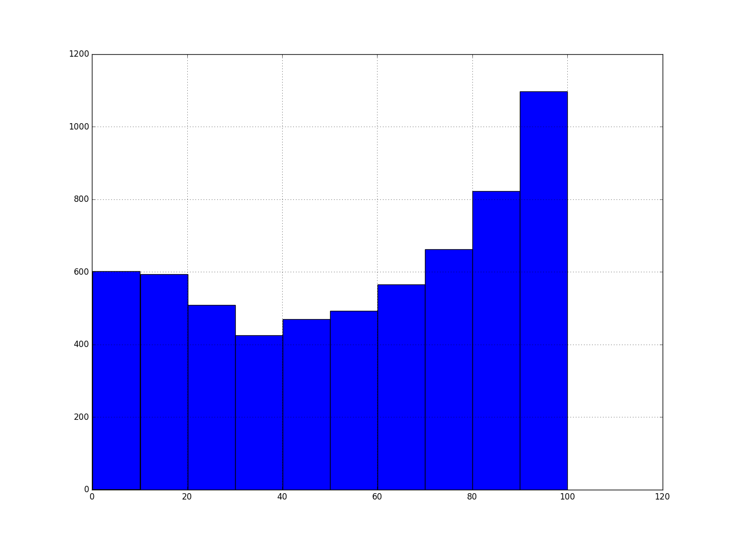
The cut-off values 0 and 100 prevent the tails from spilling past those bounds. Hence the bunching up at the ends.
Now, let’s apply it to the S&P 500.
RSI(2) applied to the S&P 500
There is actually quite a nice way to implement the RSI, using not just thresholds but the signal itself to position size.
You re-center the RSI around 50 and take positions equal and opposite in size to the RSI:
\(\mathrm{Posn}=-\frac{RSI-50}{100}\)
where I have divided by 100 to keep the position sizes in check. The look-back window for the RSI here is 2.
Applying this to the SP500 gives:
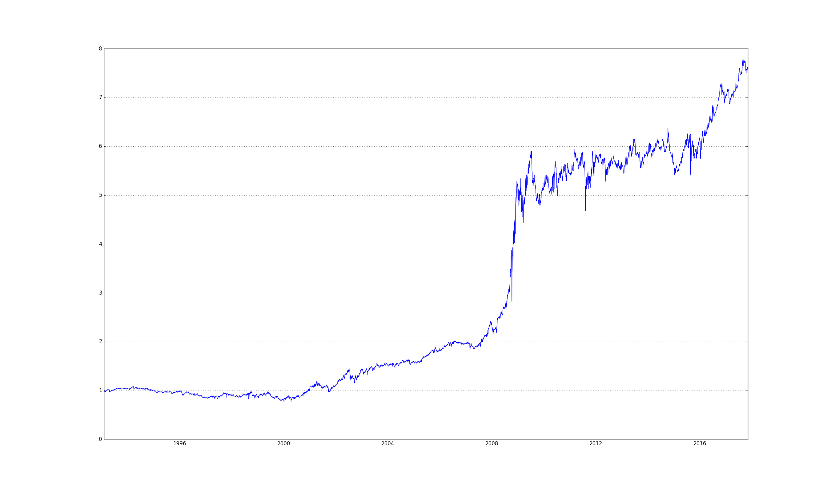
It works, but it’s quite choppy.
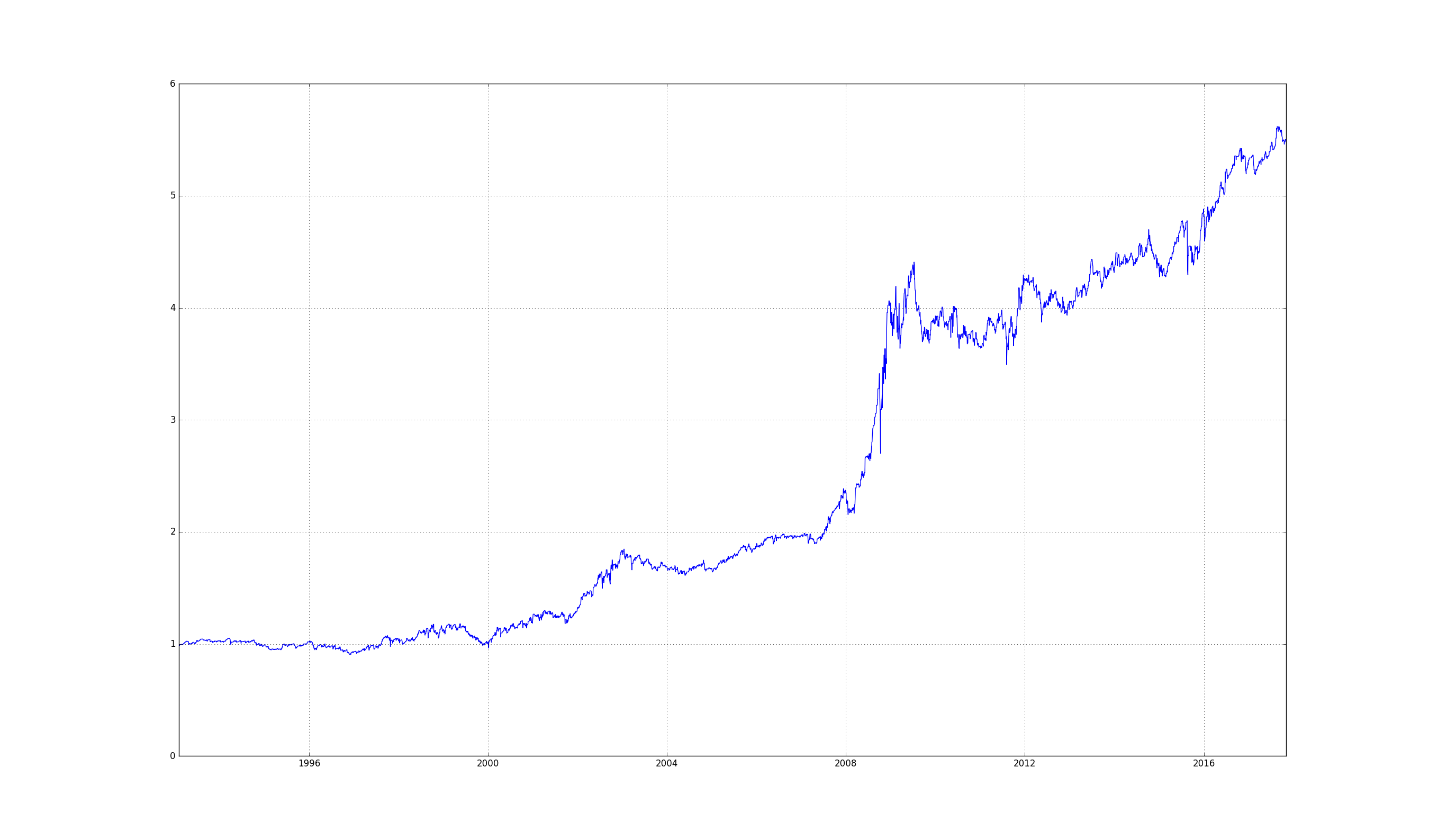
If you apply the RSI in the usual fashion, entering long / short positions when thresholds get crossed you get a similar picture. To be clear, the approach here is to only hold the S&P 500 for the following day once the thresholds get crossed. Short for high thresholds, and long for low thresholds of the RSI.
The thresholds we use are 20 for long entries and 80 for short entries.
The motivation for choosing these thresholds are that they are one standard deviation away from the mean value of the RSI (which is 50).
Mean Reversion to the 5 Day Moving Average
Of course holding only for the next day leaves a lot of money on the table.
This is where our 5-day moving average approach comes in (and it’s also Larry Connor’s exit strategy).
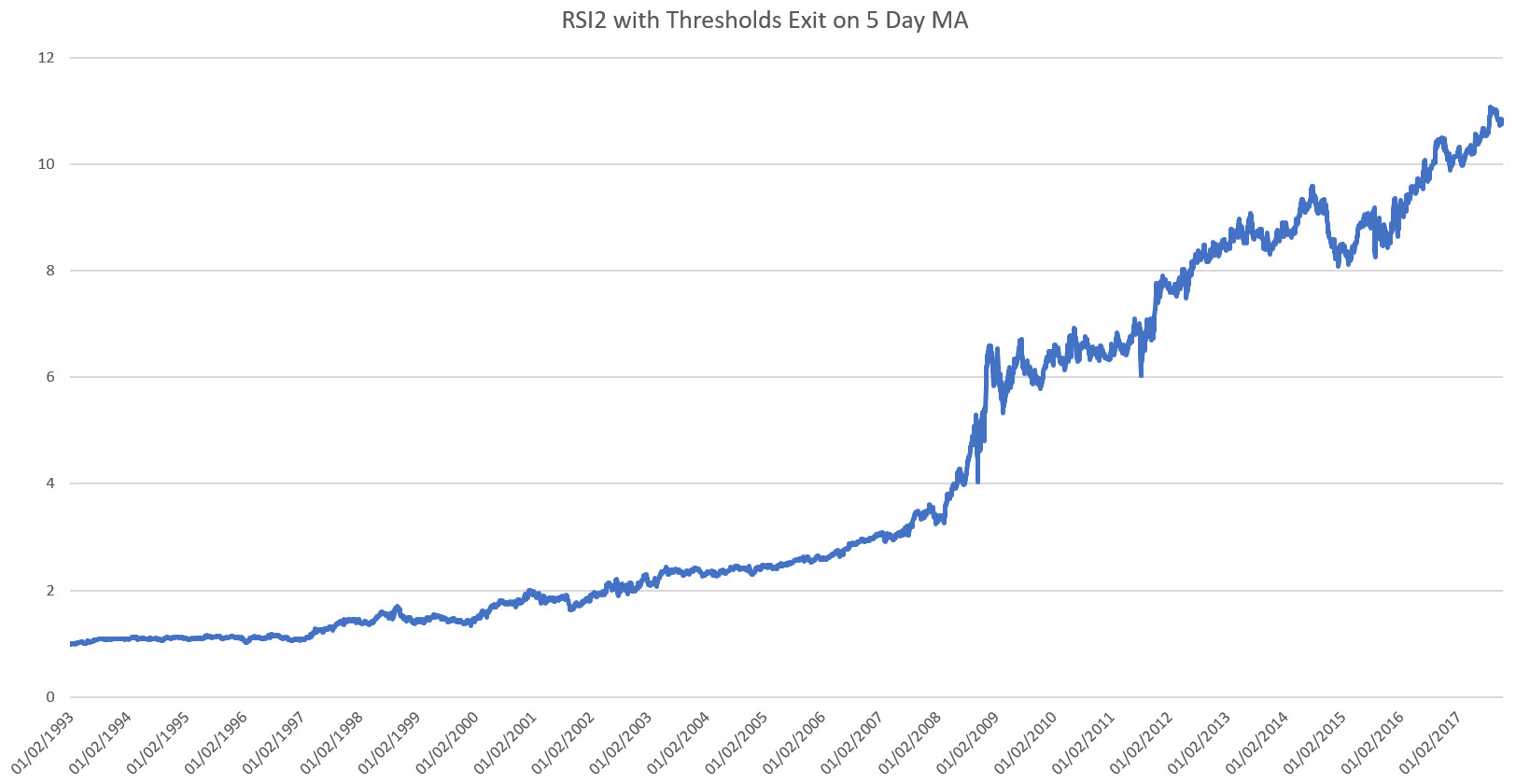
The idea here is to hold the position until the S&P 500 crosses the 5-day moving average.
If you’re long you wait for price to cross the 5-day moving average from below to above it.
And vice versa for a short position.
This approach leads to:
How can long-term momentum help?
We can now use our understanding of momentum from the previous article to add that to the mix.
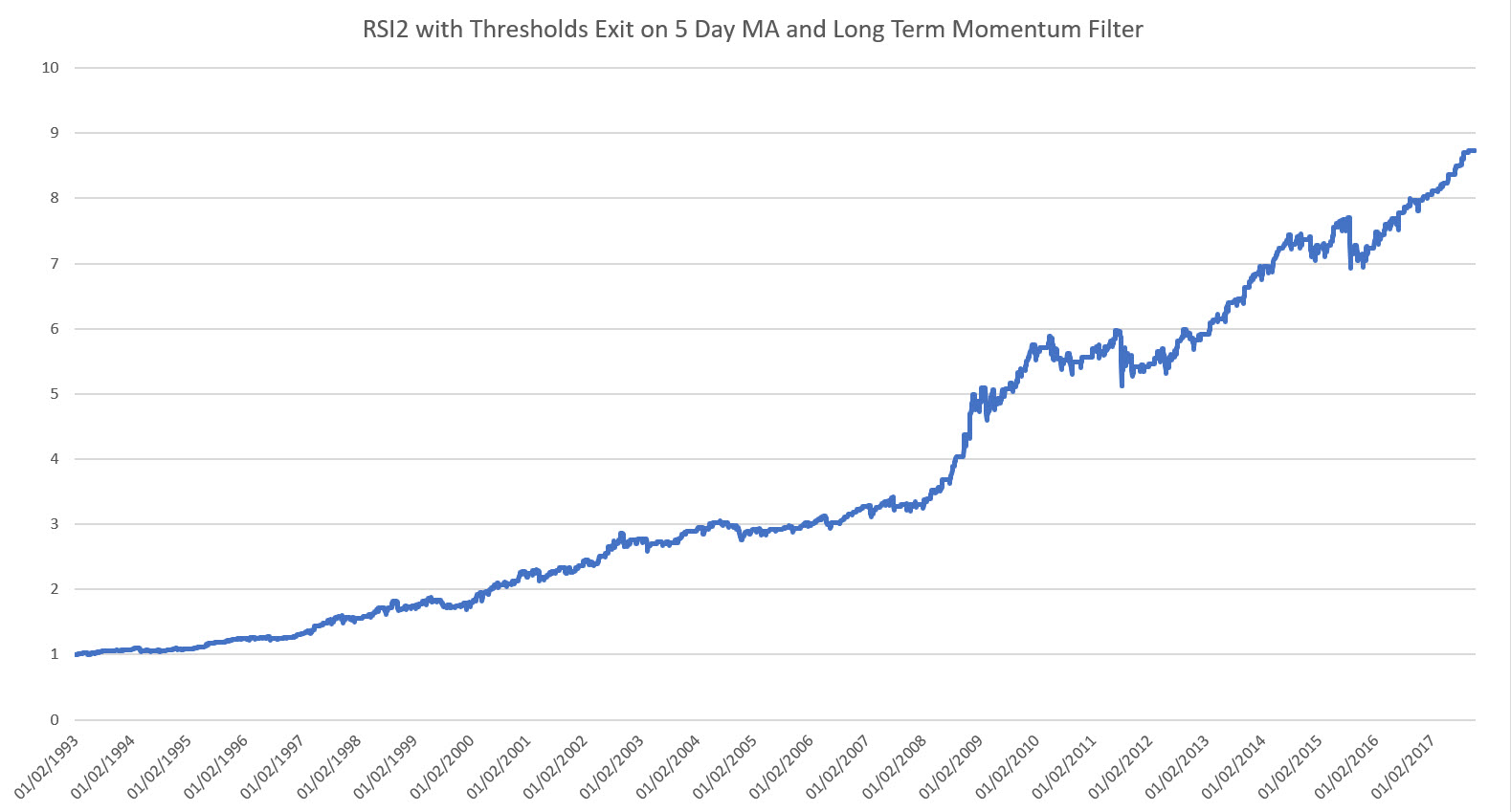
We only take on long positions in the direction of the long-term momentum, and short positions in the direction of short-term momentum.
We determine the direction of momentum by looking at the 200-day moving average. If price is above it, we take long positions, and if price is below it we take short positions.
The choice of 200 days here is to be in accord with Larry Connor’s original system. Which is not too far off the 252 business days in a year, corresponding to our 12-month momentum approach.
The resulting strategy is:
Changing Thresholds
We chose 20 and 80 as thresholds before, based on the standard deviation argument of the RSI(2) distribution.
On top of that we also saw that restricting trading in the direction of the long-term trend improved the performance significantly.
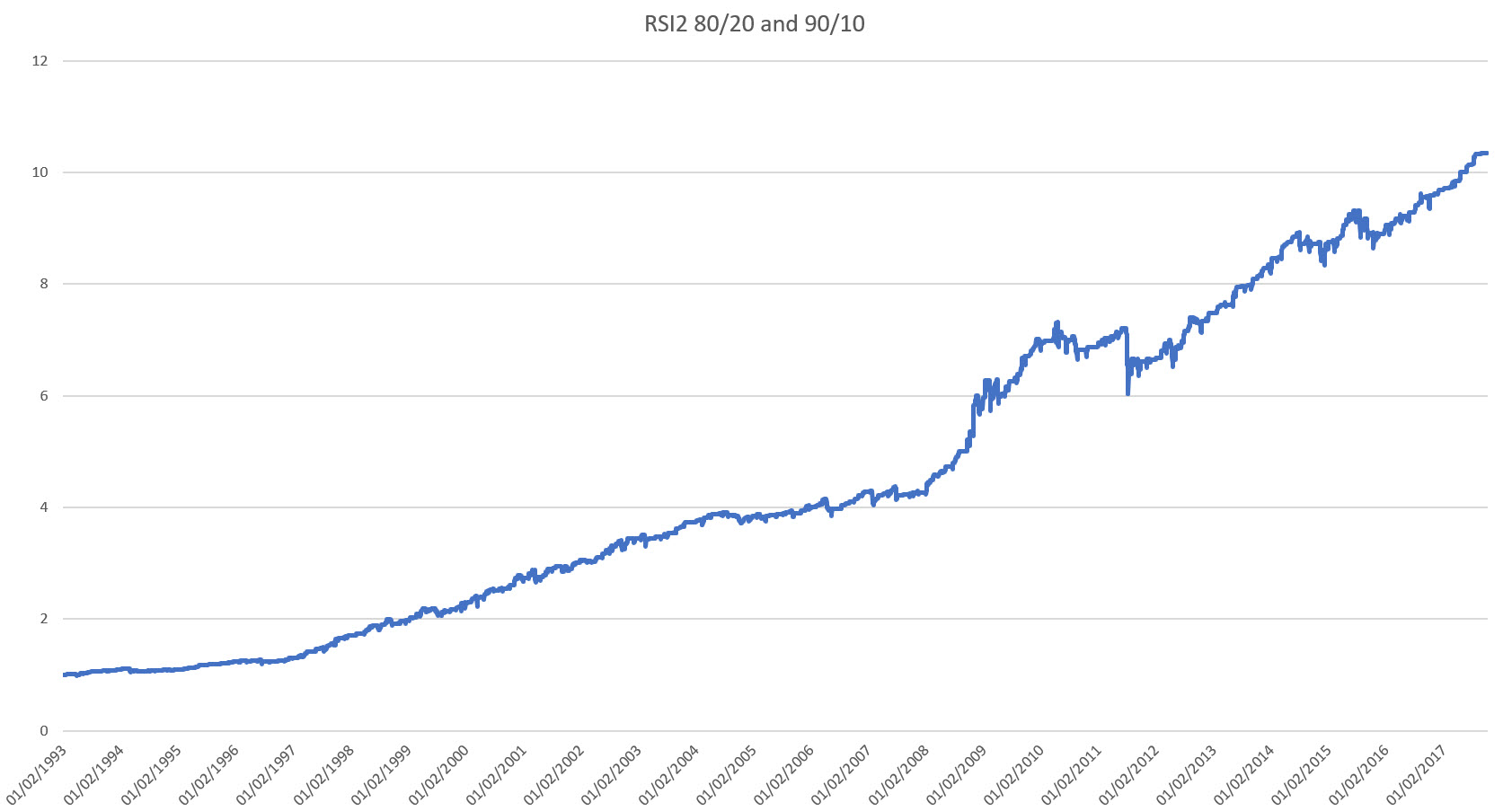
But what if we experience a divergence that continues? Of course, the usual adage is to not average down losers. However, the whole point of contrarian trading is that the further away from the mean you are the more confident you will be that you will revert to it. Therefore, the only logical conclusion is to increase position size.
The way to implement this is to layer the same strategy on top of the current one, but with thresholds set further out. I.e. at 90/10. The means that at above 80 we go short one unit, and above 90 we go short a second unit. Similarly below 20 we go long one unit and below 10 we go long a second unit.
Combining these two systems smooths out our P&L even further:
Combined with Long Term Momentum
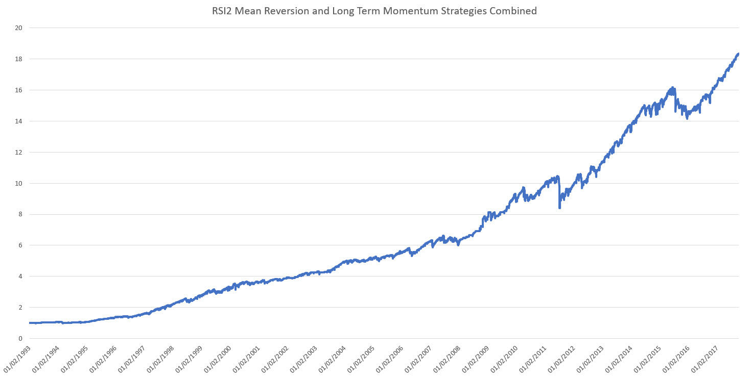
The fun now is to combine our long-term momentum system with the short-term mean reversion system and see what happens.
Right off the bat the first thing to notice is that the short-term mean reversion strategy in essence increases positions in the direction of the long-term momentum when you have dips.
You are buying dips in up trends and selling rallies in down trends.
This is a well-known approach to trading. We have managed to quantify it here.
The question is exactly how to combine these strategies. A standard approach is that of taking the correlations of the various assets/systems and optimize with respect to some criterion, e.g. minimum variance, desired return etc. (i.e. classic Markowitz).
This is complicated, fraught with statistical noise, and hence continuous rebalancing of the portfolio.
A much more straightforward method is to simply state that all correlations are zero. And assign equal risk to all assets. Under the zero-correlation assumption it boils down to risk parity.
Though this method appears naive, it is a tried and tested method of many trading desks over the decades, and has proven quite robust (as you don’t have to estimate many statistical properties!).
As long as the strategies make money, it’s a great way to combine them. Especially if you have reason to believe that the strategies are uncorrelated. If they are, your performance will improve:
Risking It Up: Properties of the Equities Mean Reversion System
As before, let’s look at some of the trading performance measures.
| RSI & Momentum | |
|---|---|
| Ann Ret | 11.1% |
| Ann Vol | 12.4% |
| Sharpe Ratio | 1.1 |
| Max DrawDown | -20% |
This is indeed a significant improvement. Our Sharpe Ratio went from 0.7 to 1.1. This alone allows a big increase on our maximum optimal leverage.
Remember, a lower drawdown and higher Sharpe ratio, lead to better leverage conditions, and ultimately to faster and greater wealth growth.
Let’s just apply half-Kelly to this strategy. In this particular case that would be a five times leverage:

All we can say is, hold on to the seat of your pants!
So Much Focus on Equities
Equities, equities, equities…
Why focus on them so much?
Because they are currently going up! Look at the charts. I always find it remarkable that people are quite willing to bang their heads against a wall, when there is an easy option staring them in the face!
Just in the last week we’ve nearly posted a 1% return on the S&P 500. And as I’ve said in the past, I’m sure a correction is somewhere round the corner. However, the markets will give you ample opportunity to move out of the way before it happens!
This was also true for 1987, using momentum measures over a variety of time horizons. The same will be true now.
Recap
This article finished the Equity bit of this series on building a consistently profitable strategy.
To recap:
- We’ve covered long-term momentum and seen it work over the last one and a half century
- We’ve covered short-term mean reversion, and granted, though it started working as of 1982, it still is going strong. No reason to abandon it.
- We saw how to combine these two to produce consistent results over the long-term
Of course, utilizing these ideas there are many more Equity assets we could explore. Such as the sector ETFs as well as international equity ETFs.
The performance will be similar within the same order of magnitude.
However, the key adage to trading is that you can’t and shouldn’t stick to one asset / system. You need to diversify.
With that in mind…
See You Next Time…
In next week’s article it’ll be back to currencies, and how they mean-revert.
The real fascinating stuff about the S&P 500 index is that it exhibits momentum and mean-reversion (of course over different time-scales).
With currencies this isn’t necessarily so. And to get to the mean-reverting juice you have to choose the right pond to fish in. Sticking firmly to the majors and their crosses we’ll construct a portfolio that has seen some consistent behavior over the last 20 and more years.
So, until next time,
Happy Trading.
If you have enjoyed this post follow me on Twitter and sign-up to my Newsletter for weekly updates on trading strategies and other market insights below!

Leave a Reply